This is Business Analytics Using Forecasting. I'm Galit Shmueli. In this video we're going to look at the third type of advanced exponential smoothing.
We already looked at simple exponential smoothing and at Holt's exponential smoothing. In this video we're going to look at Winter's exponential smoothing. And this is going to work for series that have trend and seasonality.
Remember the idea of advanced exponential smoothing is to extend the ideas of simple exponential smoothing by capturing trend, seasonality, or both. We can therefore use these methods for forecasting series that contain a trend, that contain seasonality, or that contain both. As before, the Winter's exponential method is extremely popular because it's fast and it's cheap to compute.
And we're again going to see the concepts of smoothing constants and updating equations. Recall again the types of trend and seasonality approximations that we discussed earlier. With Winter's method we'll be able to capture additive and multiplicative trend as well as additive and multiplicative seasonality.
Winter's method, also called Holt-Winter's method, and even sometimes called triple exponential smoothing, takes the idea of Holt's method and adds a seasonal component to create an even more complex system. Winter's was actually a student of Holt and he took his master's idea and extended it further. And that's why we see a method that looks similar to Holt's method, but with one additional equation for updating seasonality.
Here is what the Holt-Winter's exponential smoothing looks like. The assumption here is that our series contains level, trend, seasonality, with M seasons, and of course noise. Therefore, our forecasting equation now combines estimates of our level, of trend, and of the seasonal components.
You can see that this is an additive model, where we're using plus signs. The forecasting equation can be adjusted to incorporate either additive or multiplicative trend and seasonality. For additive seasonality we use addition to add the seasonal components.
This means that, for different seasons, we get forecasts that are different by a fixed amount. In contrast, in multiplicative seasonality you can see that we multiplied by the seasonal component. We can choose either of these equations for forecasting our series.
Notice how these two equations are for an additive trend. We're adding k times T sub t. We can adjust these to capture a multiplicative trend.
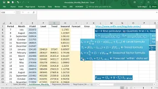
See the book Practical Time Series Forecasting for further details. In the Holt-Winter's exponential smoothing, we have three smoothing constants and, therefore, three updating equations. In the level equation, there's one part that needs an explanation.
S is a seasonal component. So when we divide Y by S, it means we're de-seasonalizing the value of Y. In the level equation, we're therefore updating the previous level, else of T-1, by adding the previous trend estimate, T sub t-1, and then combining with the de-seasonalized value of YT.
The trend updating equation is identical to what we saw in Holt's exponential smoothing. We update the previous trend by considering the latest difference between levels. In the seasonality updating equation, we see that YT is divided by the level component else of T.
This gives the de-trended value of Y. So the seasonality is updated by combining the most recent seasonal component S of T-M with a de-trended value of YT. The equations shown here are for additive trend and multiplicative seasonality.
We can create other combinations by using the appropriate updating equations. Let's return to our example of quarterly sales of soft drinks, which we saw earlier. We apply to the soft drink sales series Holt-Winter's exponential smoothing with an additive trend and multiplicative seasonality.
The software requires also specifying values for the three smoothing constants and the number of seasons. Here, we set the number of seasons to four. We obtain forecasts and forecast errors for the training period.
And for the validation period, which is the last four quarters in the series. We see that the forecasts are different for these four quarters. Taking into account both the trend and the seasonality.
Before looking at some charts and performance metrics, I'll just note that in R you can specify the different combinations of additive and multiplicative seasonality by modifying the three letter combination. In the ETS function, A means additive, M means multiplicative, and N means none. The first letter refers to the type of error, which can also be additive or multiplicative.
The second refers to the trend. And the third to seasonality. OK.
Let's now look at the performance of the Holt-Winter forecasters on the soft drink series by examining the performance charts and metrics. Looking at these, do you think this forecaster is performing well? Why?
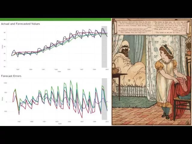
From the charts, we see that seasonality and trend both seem reasonably captured. Whether the accuracy is sufficient for our goal or not depends on the application. Our validation MAPE is 2.
26%. Is this accuracy level sufficient? Well, it really depends on how the forecasts will be used.
Notice that the validation performance metrics are much better than the training metrics. This is surprising because we typically expect slightly better training performance. Or if we overfit, then dramatically better training performance compared to the validation performance.
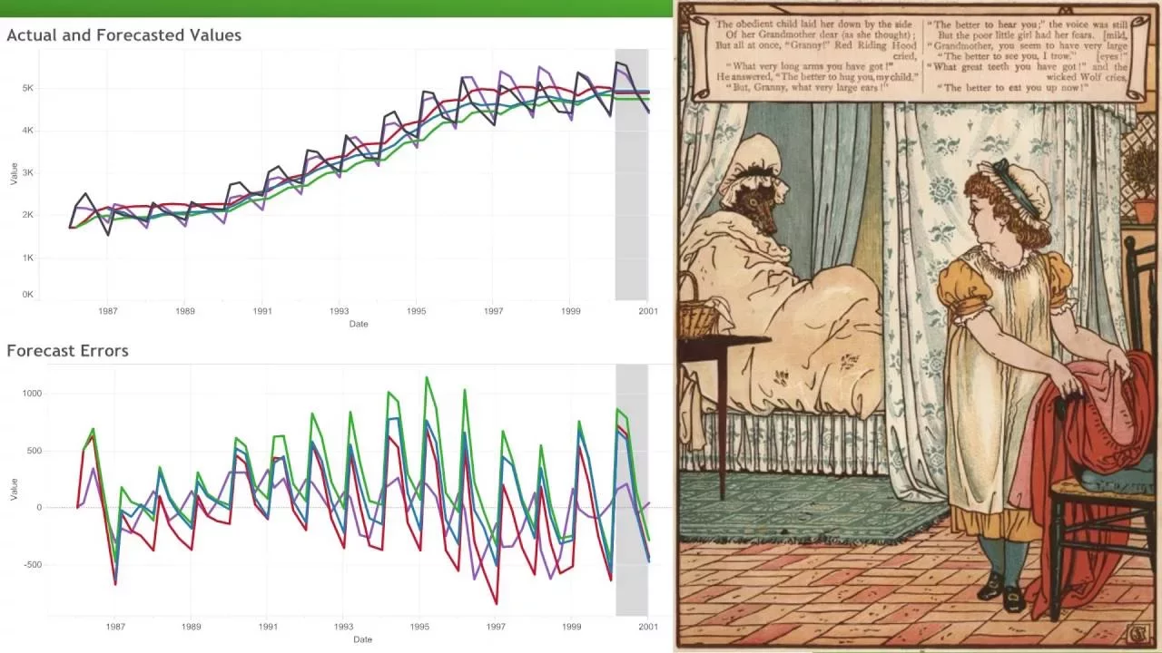
To understand what's going on, look at the charts. We see a few quarters in the training period where the forecast errors are quite large and negative around year 1997. To figure out why this is the case might require domain knowledge, especially in order to figure out whether the same reason might affect future forecasts from this model.
To summarize, by just comparing the validation performance metrics across the four smoothing methods, we see that the Holt-Winter's performs best. However, this can be misleading. We also do not see when the forecaster worked well and when it did not.
Also notice that the difference in the type of forecasted values across the four methods, moving average, and simple exponential smoothing, yield a constant value for all future periods because they do not consider trend nor seasonality. Holt's method produces increasing or, in other cases, decreasing forecasts as it considers trend, but not seasonality. Only Holt-Winter's generates forecasts that incorporate both trend and seasonality.
Here's a chart of the four methods. It's now much easier to see why and when the different methods perform as they do. The forecasts of the Holt-Winter's are the only ones that consider seasonality and, therefore, might be our choice.
In short, as in the story Little Red Riding Hood, charts are like big eyes allowing us to better see with. So the bottom line with advanced exponential smoothing is that it takes the ideas of simple exponential smoothing and extends them so that we can use them with series that have trend, seasonality, or both. Notice that we can model local additive or local multiplicative trend or seasonality.
These are patterns that might change throughout the series. The methods are simple and they're computationally cheap. That's why they're easy to automate.
We have three smoothing constants when we're talking about Holt-Winter's method and these control the speed of learning from the data. How fast do we update the level? How fast do we update the trend and the seasonal components?
If you're going to use simple exponential smoothing for forecasting a series with trend and seasonality, you first have to remove trends and seasonality. Then you can use the method and then bring back trend and seasonality. Similarly, if you're going to use Holt's method for a series that has seasonality in it, remember to first remove that seasonality, then you can use Holt, and, finally, bring back seasonality.
And, lastly, it really helps to identify the series components properly and then you can choose the right exponential smoothing algorithm from all the different choices in this family.