[MUSIC PLAYING] Welcome to Business Analytics Using Forecasting. I'm Galit Shmueli. In the next few videos, we're going to talk about a smoothing method called exponential smoothing.
In this video we'll start by talking about Simple Exponential Smoothing. The idea behind Simple Exponential Smoothing is to forecast future values by using a weighted average of all the previous values in our series. We can use this for forecasting a series that doesn't have trend and doesn't have seasonality.
If you remember, this was also the case with the Moving Average Forecaster. Simple Exponential Smoothing is very popular because it's simple, it's adaptive, and it's cheap to compute. The key concept to remember here is going to be something called The Smoothing Constant.
We're going to talk about three types of Exponential Smoothing in this course. In this video we're talking about Simple Exponential Smoothing, which is suitable for a series with no trend and no seasonality. In future videos we'll talk about Holt's Exponential Smoothing, which is suitable for a series that has a trend, but no seasonality.
And then we'll talk about Holt Winter's or Winter's Exponential Smoothing, which is suitable for series that have both trend and seasonality. Simple Exponential Smoothing, or simply SES, makes the assumption that our series only contains level, no trend or seasonality, and it does include error. So if we only have level the assumption of the Exponential Smoother is that this level will stay put and not move.
Therefore, the k-step- ahead SES forecast is simply the most recent estimate of our level at time, t. To do this, we're going to have to estimate the level. To do that we're going to use something called a Level Updating Equation.
In this equation we're taking the level at time, t and updating the previous level at time, t minus 1 by integrating information from our most recent data point, Yt. You can see that it's a weighted average where we have alpha and 1 minus alpha as our weights. Alpha is called the smoothing constant and it's a number somewhere between 0 and 1.
What this tells us is that the algorithm is learning the new level from the newest data that it's seeing. How do you start this whole system? Well, you have to initialise it with L1 at some point.
There are different ways of doing it. One option is simply setting L1 equal to the first record in your series, Y1. So why is the algorithm called Exponential Smoothing?
To see this let's rewrite the updating equation a little bit differently. We have the level updating equation as we wrote it before, but now let's substitute L sub t minus 1 with its own formula. So we start with the normal formula and then substitute L sub t minus 1 with its own formula that is based on L sub t minus 2.
We can then do the same thing again and substitute Lt minus 2 with its predecessors. And if you write this out all the way down, you'll end up with something that looks like this, alpha times Yt1 plus alpha times 1 minus alpha Yt minus 1 and so on and so forth. We see that we end up with an average of all our values in the series, but they have weights that are decaying exponentially.
Because these weights are decaying exponentially we call this method Exponential Smoothing. The smoothing constant, alpha, determines how much smoothing we do. We can take the two extremes.
When alpha is equal to one the past values have no effect on the algorithm and in fact, it's not learning anything. So the level just remains the way we started it out. The other extreme is alpha equal zero where all the values in our series have equal weight in our average.
In that case, we're not giving any more weight to more recent information. That's why we typically choose something between 0 and 1 and usually closer to 0 than to 1. Typical values that are used in industry are around 0.
1 or 0. 2, and you might see that also in software defaults. Another way to set alpha is by trial and error.
You can try a few different values, compare the predictive performance, and see which ones work better. If you do that be really careful. For example, if you're looking to minimize the RMSE or the MAPE of the training period and choosing the alpha that gives you the smallest value, you might be overfitting the training period.
So be very careful if you're going to choose alpha in that way. To feel the effect of alpha let's look at a chart that shows how alpha effects the weights on the most recent period and older periods. We can see that in all cases all these lines are different alphas, but they all decay as we go further into the past.
We can look at the actual values in the table below and you can see again the exponential decay. With alphas that are very large, like alpha of 0. 9, the decay is fast.
Whereas with smaller alphas the decay is slower. You might be wondering about the relationship between a moving average and simple exponential smoothing. There are a little bit different, but we can actually achieve results that are pretty similar if we choose the smoothing constant to be similar in a way to the moving average window.
For example, if we choose a moving average window width of w then it would be almost equivalent to using simple exponential smoothing with alpha equal to 2 over W plus 1. Another way to think of simple exponential smoothing is as an adaptive learning algorithm. Again, let's rewrite the level updating equation a little bit differently.
By opening the parentheses and reordering the components, I can write L sub t is equal to alpha times Yt plus L sub t minus 1 minus alpha times L sub t minus 1. So are one step ahead forecast, F sub t plus 1, can be written as L sub t minus 1 plus alpha times Yt minus Lt minus 1. From here we can substitute Lt minus 1 with Ft because that's exactly the forecast for time, t.
And the next step is to notice that in the parentheses Y sub t minus F sub t is actually the forecast error. So we can write that as E sub t. This last form is very simple and useful.
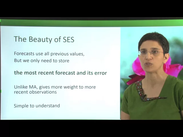
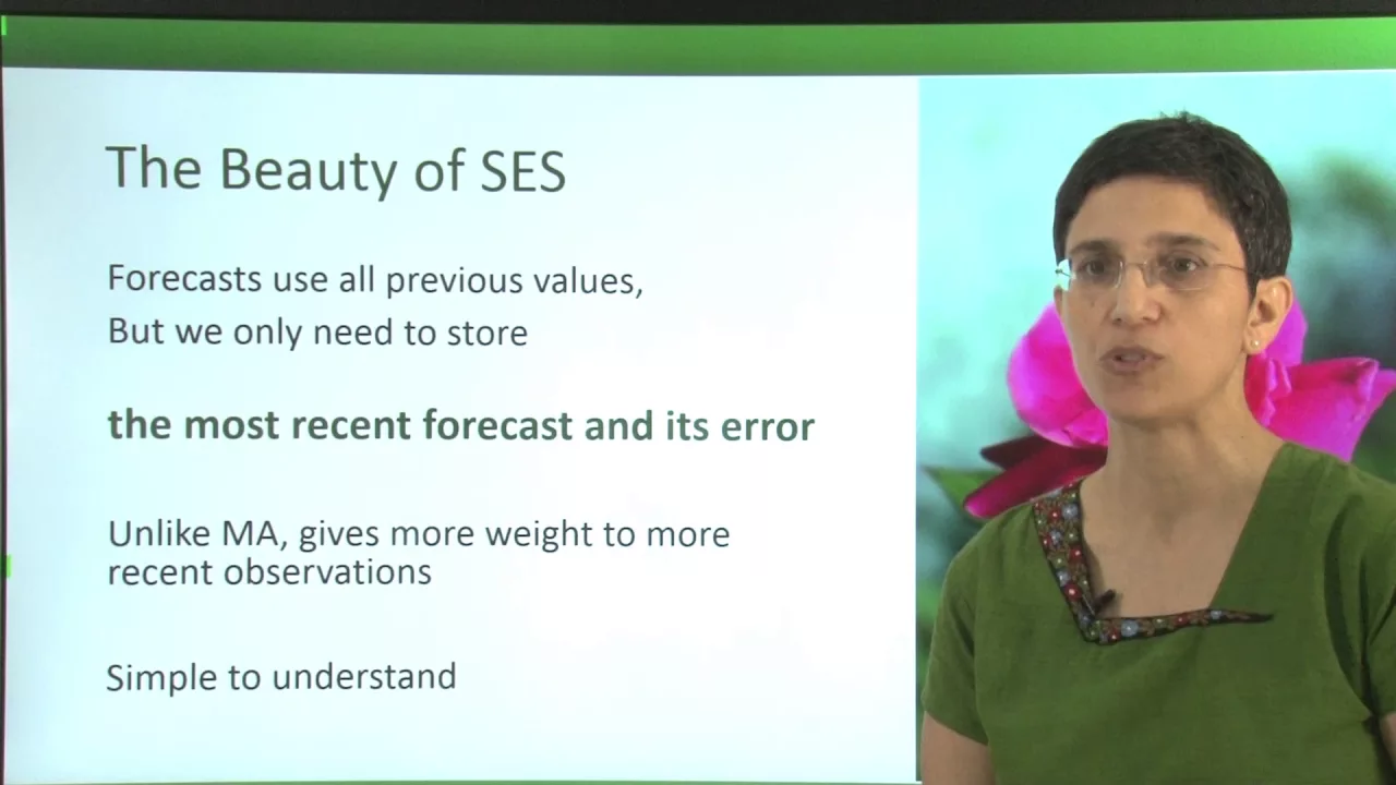
What it means is that to forecast the next time period we update the previous forecast by an amount that depends on the error in the previous forecast. This last formulation really shows the beauty of simple exponential smoothing. Forecasts use all the previous values, but we only need to store the most recent forecast and the most recent forecast error.
Unlike moving average, the simple exponential smoothing does give more weight to more recent observations. It's also relatively simple to understand, depending on which of the explanations you choose. Let's return to our example of sales of soft drinks in order to see how the simple exponential smoother works.
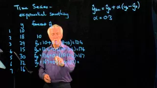
Remember that we have quarterly sales of soft drinks over a pretty long period. And now we're going to apply the simple exponential smoothing. Using the formula F sub t plus 1 is Ft plus alpha times the error, E sub t, we need the forecast and the forecast error from the previous period in order to compute the next forecast.
Let's use alpha equals 0. 2 for illustration. We therefore start with the second period in the data, quarter two of 1986.
The forecast for this period is initialised to be equal to the sales in the previous quarter. So it's $1734 million US dollars. We see that this forecast ended up being too low compared to the actual sales in that quarter, which were $2244 million.
The SES forecast for the next quarter, quarter three of 1986, takes the previous forecast 1734 and adjust it up by adding alpha times the previous error. In other words, 0. 2 times 510.
13. This gives the forecast of 1,836. 86.
The same process is repeated for the next quarter, we take our previous forecast and adjust it by adding alpha times the error. You'll notice that some of the forecast errors are negative, which indicates an over forecast. In such cases, the next simple exponential smoothing forecast will be adjusted down.
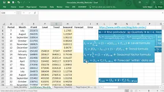
These computations can be done manually, but of course in practice we use software to compute them. In XLMiner for example, simple exponential smoothing is in the time series smoothing menu. In R we can use the SES function in the forecast package.
Looking at the performance of a simple exponential smoother for the soft drink sales, does it perform well? Why? Let's look at another example.
Remember the monthly ridership on Amtrak? This series exhibited both a trend and seasonality. What's going to happen when we apply simple exponential smoothing?
The SES forecasts are computed in the exact same way as before. We take the previous forecast and add it's forecast error times alpha. For example the forecast for March of 1991 is equal to the February 1991 forecast plus 0.
2 times the February 1991 forecast error. Looking at the performance chart, do you think this forecaster is performing well? Why do you think it's working the way it is?
The bottom line for simple exponential smoothing is that it simply takes a weighted average of all the values in our series. The weights decay exponentially into the past so that the most recent values get higher weight. The key concept of the smoothing constant is what controls how fast this algorithm learns from new data.
The SES is a simple algorithm. It's very cheap to compute because we only need to keep and use the most recent forecast and the most recent forecast error. But realize that it does not capture trend and it does not capture seasonality.
Therefore, it won't work very well if you're trying to forecast a series that has trend and has seasonality. That's what we saw in the two examples that we showed earlier. Make sure that when you're applying this method your series does not contain any trend or seasonality, or if it does, you might want to use differencing first.
In the next videos we'll look at two other types of exponential smoothing methods.