[MUSIC PLAYING] This is business analytics using forecasting. And I'm Galit Shmueli. In this video, we're going to expand from simple exponential smoothing to advanced exponential smoothing.
We're going to look at three types of exponential smoothing. We already looked at simple exponential smoothing, that is adequate for series that have no trend and no seasonality. Now we're going to look at Holt's exponential smoothing.
And this is going to work for series that have trend but have no seasonality. Later, we're going to see Winter's exponential smoothing that can handle both trend and seasonality. In this video, we're focusing on Holt's exponential smoothing.
The main idea in advanced exponential smoothing is to take the simple exponential smoothing set up and to expand it to capture trend and/or seasonality. We can use advanced exponential smoothing, either for forecasting a series with a trend or with seasonality or with both. The advantages are that these methods are very popular and very cheap to compute.
And therefore, very useful for automation. The key concepts once again, are going to be smoothing constants and we're going to have updating equations for estimating these different components. Before moving further, let's refresh our memory with the types of trends and seasonality that are popular approximations for time series.
Specifically, we have additive trend, where the trend grows or decays linearly over time. We have multiplicative trend, where the trend grows or decays exponentially over time. And we can have a more flexible polynomial trend which can capture of a variety of shapes.
Similarly, we can think of seasonality as being additive, where each season differs from another by a specific amount or multiplicative seasonality, where each season differs from another by a specific percentage. Keep in mind these distinctions when we look at advanced exponential smoothing. Let's think about our series as, again, comprising of two parts, a systematic part that includes level trend and seasonality and a non-systematic part that is simply the noise.
When we talk about additive models, we're taking our series and breaking it down into the different components by adding them with summation signs. In contrast, when we're talking about multiplicative models, we're taking our series and dividing it or decomposing it into the different components, but then, combining them by multiplication signs. This is the main difference between the two types of models.
First, we'll talk about Holt's exponential smoothing, also sometimes called double exponential smoothing. The idea is to take simple exponential smoothing but to add a trend component. Before we talk about the method itself, let's think about what it means.
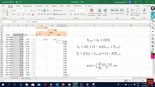
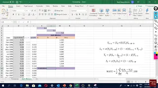
We're making an assumption here that the series has a level, it has trend, and of course, it has noise, but there is no seasonality. Therefore, when we're talking about the forecast, we're going to take an estimated level and combine it with our estimated trend at the most recent time point. This is our most recent level estimate and our most recent trend.
And K is how many steps into the future we're trying to forecast. We're going to have to updating equations, one for the level and one for the trend because we're learning both of them from the data. The updating equation for level is similar to what we had in simple exponential smoothing.
We're going to take the most recent data point and use it to update our previous estimate of the level at time T minus 1. The only difference is that here we also add the trend and take it into account. What this equation is showing us is that we're basically adjusting the previous level by adding a trend.
The second equation is going to update our estimate of the trend. So we're going to take the trend in the previous time period and update it by looking at the difference between the most recent level estimates. Were updating the previous trend by using the difference between the most recent level values.
Notice that this setup allows the trend to vary and change in shape over time. You also notice the smoothing constant beta here. And beta is controlling the speed of adjusting the trend.
So if the trend changes very quickly during the series, we might want to learn it faster. How do we choose the smoothing constants, alpha and beta? We can use default values that most software will have.
Those are based on empirical experience and you'll typically see values in the range of 0. 1, 2 or in that range. The other approach is to try and find alpha and beta that minimize some error metrics, such as RMSE or MAPE or any other type of metric over the training set.
If you do that, you have to be careful of overfitting. Because if you use those optimized alpha and beta, you might not be able to generalize very well into the future. Recall the two types of trend approximations, additive and multiplicative trend.
We can adjust the Holt exponential smoothing forecast formula to capture either an additive trend or a multiplicative one. For an additive trend, we use an addition sign in the formula. We add to the current level, L sub T, the estimated trend multiplied by the number of steps ahead, K, that we are forecasting.
As we forecast further into the future, the trend effects the forecast to a larger extent. Now let's look at a multiplicative trend. Here were multiplying the current level by the trend.
And the number of times we multiply by the trend, depends on the number of steps ahead, K, we're forecasting for. This means that it's a good idea to first identify the type of trend in your data, such as by using visualization, and then choosing the appropriate Holt exponential smoothing algorithm. Let's now see an example.
Recall the quarterly sales of soft drinks that we saw earlier on. These were the quarterly sales of soft drinks in North America in millions of US dollars. We have data from the first quarter of 1986 to the first quarter of 2001.
Here's the output from applying Holt's exponential smoothing with an additive trend to the soft drinks data. Unlike moving average and simple exponential smoothing, it's no longer so simple to obtain the forecasts from the three columns that we used earlier. It's definitely advisable to use software for generating the forecasts and errors.
In XLMiner, we can use the double exponential function in the time series smoothing menu. In R, we can use the ETS function in the forecast package. Notice how the forecast for the validation period are no longer constant for all four quarters, unlike the moving average and simple exponential smoothing forecasts.
This is because the Holt forecaster assumes a trend and it uses that trend to tune the forecasts into the future. Let's see how well this forecaster performed. Take a look at the forecasts, the red line in the top chart, and take a look at their errors in the bottom chart.
Would you say that this forecaster is performing well? Why? As in the moving average and simple exponential smoothing examples, we see that here too, seasonality is not captured.
However, the trend is captured much better. There is no more lagging behind effect and the forecast error chart doesn't have an apparent trend. But can we do better for these data using Holt's exponential smoothing?
Well even if our series does contain seasonality, we can still use Holt's exponential smoothing if we remove the seasonality first. So our first step will be to remove seasonality, which we also call to de-seasonalize a series. We've seen one method of doing that.
For example, we can use differencing. In this example, we have quarterly data so we might use a Lag-4 of differencing to remove the quarterly seasonality. We then take this de-seasonalized series and to that, we can apply Holt's exponential smoothing.
We generate forecasts but then, we have to bring back seasonality into those forecasts. And that is called to re-seasonalize the series or the forecasts. How do we do that?
Well, we're going to have to reverse the operation that we did in step one. So if we use differencing in step one, we're going to use un-differencing at the same lag at step three. One important point to notice about different exponential smoothing algorithms, when we're using different software packages or even the same software package, but different versions of the software, the implementation can actually make a difference.
So don't be surprised if you find different forecasts or different forecast errors when you're using different implementations. Let's see one more example, this time comparing a fixed validation period to a roll forward validation. In the first case, we'd be interested in forecasting monthly Amtrak ridership in the next 12 months.
In the second case, we're interested in forecasting one month ahead for the next year. Here's the first case. We can apply Holt's exponential smoothing with alpha equals to 0.
2 and beta equals to 0. 15, these are the software defaults. And we're using these to forecast the last 12 months in the series, which are in the gray area.
We see the forecasts are linearly decreasing. Now let's look at a roll forward scenario where we update our forecast each month. The training period looks identical to the first scenario.
However, in the validation period, we see a completely different picture. This is because we are updating our forecasting month by month. The bottom line for advanced exponential smoothing thus far, is that we're going to extend the idea of simple exponential smoothing to series that also contained trend, seasonality, or both.
We looked at Holt's method which can capture an additive or multiplicative trend. We talked about two smoothing constants, alpha and beta, which control the speed of learning of the level and of the trend. And we discussed software implementation and how we can get different results by using different software or different versions.
These methods are very simple and cheap to compute and therefore, you might see them automated in different software. Finally, notice that it's very useful to identify the components of the series so that you can properly choose the right exponential smoothing algorithm for your data.