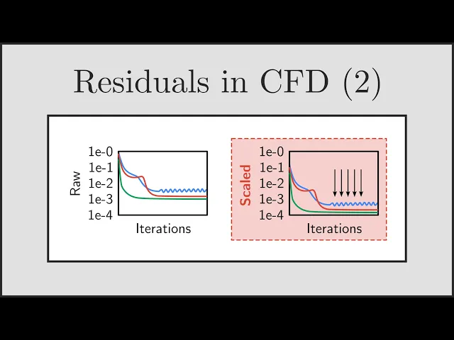
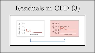
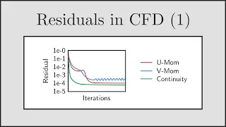
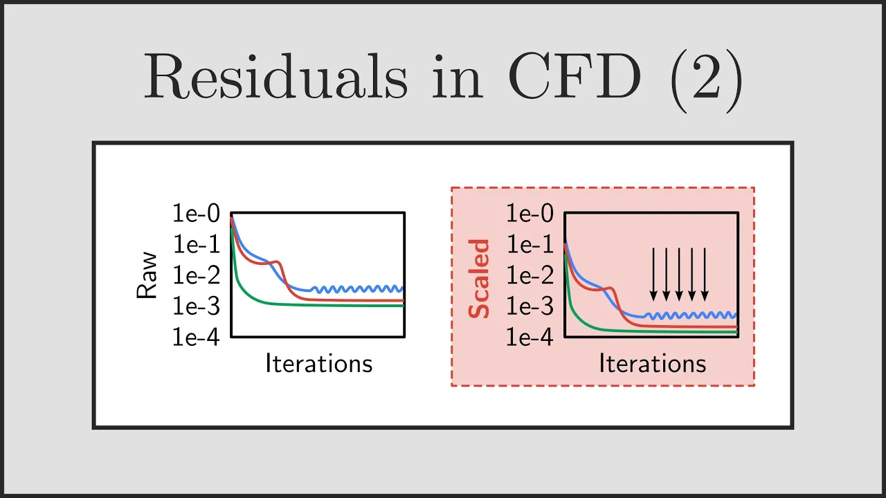
welcome to part two of my lecture series on residuals in cfd in part one of this lecture series we looked at basic residuals what they physically mean and how they're calculated by cfd codes now if you've taken a look at the user manuals and in online forums for cfd you'll often find things referred to such as scaled residuals normalized residuals and relative residuals and this can be quite confusing as it's not clear what these terms actually physically mean and how they're calculated by cfd codes i'm going to clear up a lot of this confusion in today's talk by talking about scaling residuals i'm going to go through the process and explain to you why residuals are scaled why we need to do this and how the scaling process is actually carried out by cfd codes so by the end of this talk you can have an even deeper understanding of what residuals are which is ultimately going to help you when you're assessing the convergence of your own cfd cases and general understanding of cfd codes in general so let's jump straight into the talk so let's start things off with a quick recap of what we talked about in part one of this lecture series now you'll remember that we looked at the simple example of 1d heat conduction in a bar where we have a 1d bar and at both ends of the bar we have a fixed temperature on the left side we've got a hot temperature and on the right side we've got a cold temperature and we've got no heat sources in the bar for this example and when we divide the bar up to foot into four elements we find that the temperature profile of course varies linearly between the hot and the cold end of the bar and heat will flow from the hot end of the bar through to the cold end of the bar and we could solve this problem analytically by hand but the way we chose to do it to show how cfd codes work is we used the finite volume method and we applied conservation of energy for each individual cell in the mesh and resulted in a matrix equation a t equals b and solving that matrix equation will give the temperature t1 t2 t3 and t4 at the centroid of each of the four cells in that mesh now you'll also remember that cfd codes generally use an iterative process to calculate the solution for the temperature equation and the other equations that are solved and so what that means is that at any particular iteration in the solver the solution does not match the final solution and a way that we can think about this for our temperature profile is that when we have no heat sources in the bar we expect the temperature profile to vary linearly between the hot and cold ends of the bar but while we're converging that temperature profile will not be linear and so what that means is if we think of any particular cell now the gradient of the temperature profile while we're converging between those two adjacent nodes will be linear but it won't match through the left and the right faces of the cell and of course what that means is that because the gradient is different that means that the heat flux out of the left face of the cell and the right face of the cell don't balance and so we have a local energy imbalance in each of the cells in the mesh while the code is converging and what we can then do after we've solved a particular iteration in our iteration process is we can take the current solution for that temperature vector t1 t2 t3 and t4 and substitute it back into the equation a t minus b and that will calculate the residual vector for us which is uh here on the slide for the four cell mesh r1 r2 r3 and r4 where each of those r values gives the local energy imbalance in each cell in the mesh and of course as the solution proceeds and the iterative solution gets closer to the final solution those energy imbalances will reduce towards zero and when those energy imbalances are reduced below some certain tolerance we can be happy that our solution is iteratively converged to some tolerance now the focus of today's talk is going to be taking that idea of the residuals and applying a process called scaling to the residuals and what i want to do before showing you the process is to explain to you why we need to scale the residual vector and the way i'm going to do this is just by considering two very similar examples which you can see here on the slide in both cases we've got the same case that we looked at before we've got the 1d heat conduction in a bar between two fixed temperatures and for the case on the left i've got the hot end of the bar at 31 degrees c and the right end of the bar at 30 degrees c so a very small temperature difference there only one degrees and in the case on the right uh i've got the temperature of the left end of the bar is really hot say 200 degrees and the temperature on the right is 30 degrees and so of course because the wall temperatures are different we expect the gradient of that final solution to look different when we solve the problem and in both cases we've got no heat sources in the bar so we're still going to get a straight line variation of the temperature between the two sources now of course because the temperature difference is very small in the left case the gradient's going to be very shallow whereas in the right case the gradients can be a lot steeper now suppose that we were carrying out an iterative solution process and we looked at the solution during a particular iteration in that iteration process and if we look at the case on the left for example firstly and we were to look at those heat fluxes out of the left and right faces of the cell for that cell that's shaded in gray you can see that through the left face of the cell we've got heat flux of 0. 1 watts and then out of the right face we've got a heat flux of 0. 11 watts now of course there's a local energy imbalance here and that energy imbalance is the residual which for the case on the left is 0.
01 watts it's just the difference between the heat out of one side of the mesh and then the heat flux out of the other face of the cell in the mesh now if we just flick over and look at the case on the right we do exactly the same thing again but in this case for example we've got 100 watts coming through the left face of the cell and we've got 100. 01 watts coming out of the right face of the cell now again the difference between those two fluxes gives us the energy imbalance which is the residual for that particular cell and in this case we also find that the residual is 0. 01 watts so for both of these examples we can see that those cells in the mesh have the same residual but the question for us as a cfd analyst is are both of these cases equally close to convergence because we use the residuals to judge convergence at the moment and both of these cells have the same residual so are they both as close to convergence as each other now the trick and what you'll notice is that actually if you compare the energy imbalance in that cell or the residual relative to the flux of energy through that cell what you find is that the residuals are actually very different so if you take the case on the left and we've got a residual of 0.
01 watts but then if you divide that by the flux of energy through the cell which is 0. 1 watts you find that the as a percentage the energy imbalance is ten percent so of all the energy that's passing through the cell ten percent is being lost because we're not yet converged we've got a relative or percentage uh energy imbalance of 10 in that particular cell whereas if we look at the case on the right we've still got the same residual 0. 01 watts we've still got the same energy imbalance but relative to the 100 watts of energy that's passing through that cell the scaled residual is only 0.
01 percent so the case on the right is actually a lot closer to convergence because the the energy imbalance relative to the total energy passing through the cells is a lot smaller and this concept is actually what a scaled residual is so you can think of a scaled residual as the percentage of energy lost or gained in a particular cell in the mesh during the iteration process so that's the basic idea now we're going to expand on it a bit more and think about maybe how that might be calculated now before i do that i just want to put a quick flag in to remind you all that i'm just considering the energy equation in this particular talk but the same idea can also be applied to the other equations that are solved iteratively by the cfd solver so if you were to solve the u momentum equation for example using the same approach you'd find there'd be a residual in each of the cells in the mesh and that residual represents the local force imbalance in that particular cell in the x direction so you can see in the small image on the right we could have just applied this same idea to the u-momentum equation where we'd have 30 newtons of force acting on the left face of the cell and 30. 01 newtons acting on the right face of the cell so in that case the residual is 0.