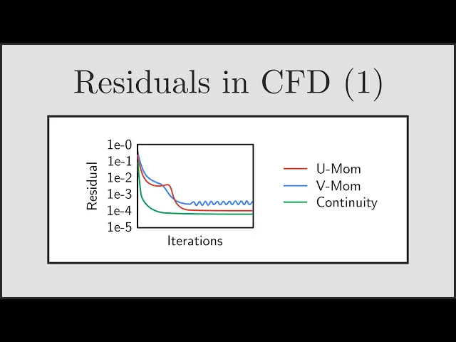
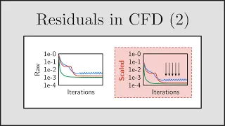
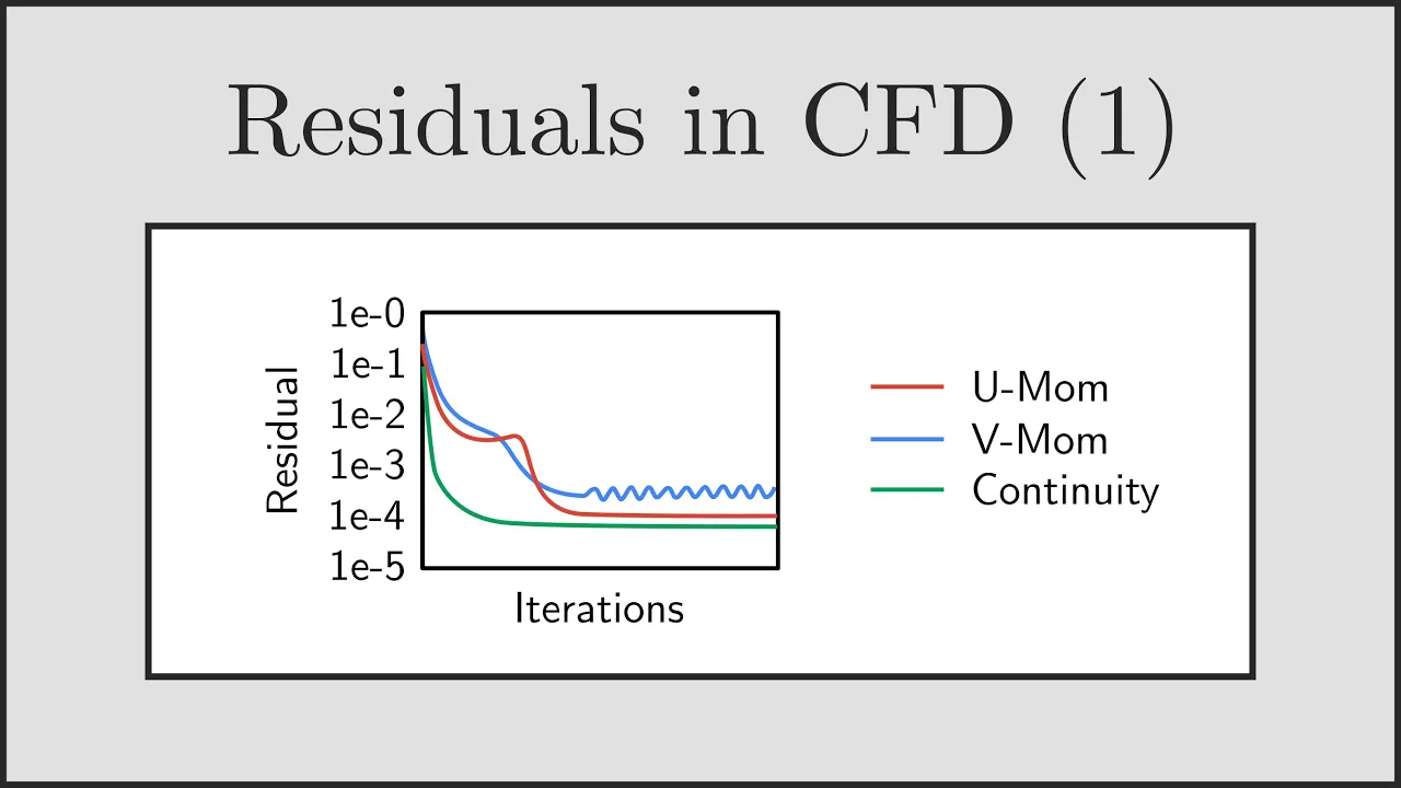
if you've been carrying out your own cfd simulations then you're probably used to looking at plots of residuals which look something like this now there's a lot of confusion around residuals what they actually mean and how they're actually calculated particularly because different cfd manuals often give different explanations use different notation and use different terminology for residuals and imbalances and it's not clear exactly what's going on this is even more difficult when you're trying to assess the convergence of a real cfd case and you're not sure if your cfd simulation is sufficiently converged or if there are any errors and whether those errors are important now what I'm going to be doing for you today is going through a series of talks on residuals in cfd this is going to be a four-part series where I'm going to go into detail about residuals and more specifically I'm going to be providing you with physical understanding so you actually know what residuals really mean when you're looking at them I'm going to be contrasting that with uh imbalances um and I'm also going to be looking at things like scaling and normalization of residuals as well so that you understand the nuances and how different representations of the residual are different and how they vary between different cfd codes all of this is going to culminate in the final part of the series where I'm going to give you some techniques which will help you assess the convergence of your own cfd cases and and really give you a fresh look at how you're assessing your cfd simulations this is going to be a fantastic set of talks let's jump in now with part one where we're just going to look at the basic idea of residuals and to understand exactly what it physically means now rather than diving straight into the mathematics behind residuals what I'm going to be doing is going through an example problem so that we can help develop some understanding of what residuals physically mean first and then we can go back and look at the mathematics later now the example problem I'm going to be using is simple straight forward 1D heat conduction in a bar between two fixed temperatures on either side and you can see this in the diagram on the slide we've got a hot surface held at some fixed temperature uh connected to a cold surface again at another fixed temperature uh connected by a 1D bar or rod and we dividing that bar or rod up into four cells or four elements of course we could divide the rod up into as many cells or elements as we wanted but for this talk and for Simplicity we're just going to use four volumes now because those two surfaces are at different temperatures we're going to get heat flowing uh from the hot surface through to the cold surface and that's what we're interested in now this is a very simple problem we're only considering heat conduction but it's sufficient for us to understand what residuals are and how they're developed and of course we can apply that same process to look at other transport equations that are solved by the cfd code now this is a very simple problem and the solution is actually very straightforward and we can get analytically if we wanted to if there are no sources of heat in the bar so we've just got those two fixed temperatures on either side then we'll get the solution which you can see on the left and the resulting temperature profile across the bar will be linear of course now if there are sources of heat in the bar that temperature profile will be nonlinear and the temperature profile may look something like the image you can see on the right there and in both cases we we don't actually need to solve this problem uh numerically if we wanted to we could do this with a with a hand calculation but for now it's a very useful example it's very simple so that we can start understanding what residuals are and where they come from now what we're going to be doing is just setting up a system of equations so we can solve this problem numerically and then when we've got that we can start to see where the residuals come in and what they actually mean and the way we're going to develop the numerical equations is by considering conservation of energy for a single cell in the bar and if you consider the second cell from the left in the bar as you can see in the diagram then for that particular cell we can have uh heat conducting out of the left face of the bar we can have heat conducting out of the right face of the bar and we could also have a source of heat in uh that section of the bar from some kind of internal heating mechanism for example and if we apply conservation of energy to that cell we can use fia's law to get the heat flux across the left face of the cell and the right face of the cell using the temperature difference uh across um across that cell face using the equation you can see there on the slide and the simplest way to develop us uh an equation for conservation of energy is to start with equation one so the heat flux across the left phase plus the heat flux across the right face plus the heat Source will of course equal zero and then we can use furry as law and substitute in for those the heat flux the heat flux across the left face and the heat flux across the right face and you'll notice there that we've uh assumed that the temperature uh profile between those two cell centroids is linear so DT by DX will just be the temperature difference divided by the distance between those C centroids Delta X and then we have k and a and there the thermal conductivity and the face area of that face of the bar so that gets us to equation two and then the next trick and what we're going to do is just rearrange equation two and you you can go ahead and do this uh yourself if you want to uh at home we just going to rearrange it in terms of the unknown temperatures T1 T2 and T3 where those temperatures are just the temperatures at the centroids of the cells in the bar and when I'm numbering those left to right so the first C cell is T1 the second cell is T2 that's the one we're currently interested in then T3 and then T4 so we've got this rearranged equation three in terms of those unknown temperatures T1 T2 and T3 of course this is a this is a a linear algebraic equation and what we can do to just simplify this equation for now equation four is we can just take those uh multipliers in front of T1 T2 and T3 and just write those as coefficients a 1 a21 a22 a23 Etc just to simplify things and make it easier for us to fit on the slide but those coefficients a just represent uh those collection of thermal conductivities areas and uh distances Delta X so now we've written conservation of energy for cell 2 from that previous slide we could go ahead and do exactly the same process and write conservation of energy equations for the other cells in the mesh and of course we'd have to do something slightly careful at the boundaries to make sure we got those bound temperatures in but generally we'd be able to write four equations equations 6 Seven 8 and 9 you can see there on the slide and those four equations are in terms of four unknowns the unknowns being the temperatures at the centroids of each of those cells in the bar so got T1 T2 T3 and T4 and what the set of equations is physically representing is the heat conduction between those cells in the bar because of course the heat can only conduct to a cell on either side of our cell and then that term B on the other side is just going to give heat sources if there are any and any boundary conditions affecting that cell in the bar now of course with four equations in four unknowns we can write that quite concisely in Matrix form uh a t equals B which you can see there in slide 10 and this is a fantastic position we're in now to get a numerical solution because we can use a a linear algebra solver to solve for the unknown temperature Vector that's T1 T2 T3 and T4 which when we solve the equation will give us the temperature at the centroids of those four cells in the bar and of course those of you who are used to linear algebra will notice that uh the length of the temperature vector and the size of the matrices in this case is equal to the number of cells in the mesh so we've got four cells but if we had six cells or eight cells for example our temperature Vector would be larger and the size of our Matrix problem would go up but in general uh we have one equation for each cell centroid in the bar that we're considering so let's suppose we went ahead and did that and we filled in our a matrix and our B Matrix and we passed that system of equations over to a linear algebra solver and we were able to calculate the temperature Vector T1 T2 T3 and T4 and you'll notice in this solution now that we've plotted it that the temperature variation between the centroids is l linear and the reason it's linear is when we set up that system of equations and we used fia's law we assumed that the temperature uh the temperature variation between the centroids was linear so that DT by DX would be the difference in temperature divided by the distance so we've got this piecewise linear profile between the temperatures uh in the bar and of course the end temperatures will be equal to the temperatures of the hot wall and the cold wall now once we've solved uh the equation and we've calculated that temperature profile in the bar the next thing we can do is we can actually go back and back calculate the heat fluxes across each of the faces uh of the cells in that mesh and the way we would do that is by once again using Fu's law and in the example you can see here on the slide for example if we wanted the heat flux across the right face of that cell what we would do is we would take the temperature difference uh across that face and then multiply that by Ka over Delta X and just as a quick reminder the minus sign is in there of course because heat flows in the direction of the negative temperature gradient so from hot to cold that's the direction that the heat Flows In which is the reason why you've got that negative sign in there so we could go ahead and use fia's law once again and we could calculate the heat fluxes across all of the faces uh in the mesh once we've calculated our temperature profile F so that would be a postprocessing operation that we could do to calculate the heat fluxes across the faces now that approach that I just went through there was using a very direct approach using a single step passing the system of linear algebraic equations to a a solver which would then in one step calculate that temperature profile for us using um using some kind of solution method and we'd get that in one overall iteration of the solver now in general C FD codes use an iterative approach to calculate the solution where it may take multiple attempts to solve that temperature equation uh being coupled or not coupled with the uh the fluid equations for example and maybe some other uh equations of species transport and so for that reason because we're using an iterative process to solve this system of equations uh it takes us several iterations to calculate that final temperature profile and what I want you to do is think now of the case where we have that heat conduction in a bar between two fixed temperatures but with no heat sources in the bar now for that case uh the final temperature profile will of course be linear between those two temperatures and you can see that in the plots on the slide given by the dashed line now before we achieve that final solution of course with an iterative approach we calculate a solution that's approximately uh what we think the temperature profile might be and until we achieve convergence that temperature profile uh will not be the same as the final converg solution and what you can see here on the slide is that if you were to plot that temperature profile every iteration or every few iterations you'd find that as you get closer to convergence the temperature profile uh approaches that final linear profile which you of course know is going to be the final solution and what we're actually interested in when it comes to residuals is not necessarily the final solution which you can see there in the plot on the right but what's actually happening in the plots on the left so we've got a temperature profile but it's not uh necessarily the same as the final temperature profile and there's some error here that's actually what we're interested in when we're looking at residuals now if we think about these temperature profiles in a bit more detail what we see is that of course the final solution the temperature uh the temperature profile is linear and that means the temperature gradient for this example at least is constant so if we looked at the gradient of that uh slope between each of the points or between each of the cell centroids what we would see in the image on the right is the when the solution is fully converged that gradient will be equal along the line so the gradient and therefore the heat flux along that bar will be equal between all of the cell centroids now before we've converged we may have some random temperature profile that doesn't uh necessarily agree with what our final solution is and if we look at the gradients between those points we can see that for this example the gradients don't match and that's a really interesting observation that will help us to understand residuals now for that case on the left because the temperature gradient doesn't match on each sides on each of the sides of that centroid that also means that the heat flux doesn't match out of both size of the cell so I want you to think back to the cell now and for this example we've got no heat source is in the cell and so that must mean for us to satisfy conservation of energy the heat flux out of one side of the cell will be equal to the heat flux coming in from the other side of the cell for energy to be conserved but for this case on the left you can see that before we reach cons uh convergence of our solution because that temperature gradient doesn't match the heat fluxes also don't match so that means we're not satisfying energy conservation until we have convergence so the next question is if we're not satisfying conservation of energy where does that missing energy go while we're while we're converging and to answer that question we need to think back a little bit to what is what we've actually done to get to this point and you'll remember that each of the rows of the Matrix equation that we set up represents conservation of energy for a particular cell in the mesh so the second row for example represents conservation of energy for the second cell the third row will represent conservation of energy for the third cell and so on and so each of those rows actually represents that full equation for conservation of energy that I have there in the red box but it was just rearranged a bit in terms of the temperatures it still represents conservation of energy so what we need to do is actually go back to that original equation for conservation of energy and add an additional term that captures this missing energy which we have uh when we're solving with an iterative process we've got some missing energy that we need to satisfy conservation of energy it may be uh positive if we have an energy under prediction or it may be negative if we have an energy over prediction and you can see there in equation 11 I've added this extra term in and called it uh r or R2 to be more specific because this is the missing energy or the residual for cell 2 so now with this additional term this residual added to conservation energy that equation 11 will be satisfied and we have accounted for all of the energy and we're not missing any and so what we can see here is that the residual physically represents the local energy imbalance or the missing energy for a particular cell in the mesh that's what it physically represents and of course we could repeat this process and rewrite our conservation of energy for all the other cells in the mesh we could rewrite it for cell three and cell one and cell four adding this extra term called R to each of those equations and this would allow us to arrive at the set of equations you can see there on the slide 13 through to 16 all we've done is just added an additional term to each of those equations to represent the the missing energy or the the energy imbalance and of course this set of equations can also be written in Matrix form and that allows us to arrive at equation 17 we've now rather than having a t equals B we've now got a minus b equals R and that R there is the vector of residuals for all of the residuals uh in the mesh now of course we could have arrived at equation 17 slightly differently if you wanted to use more of a direct approach you could have just noted that because when we're not converged a t doesn't equal B you could just subtract B from both sides and then the small quantity left over you could assign uh to the residual Vector R but I prefer to think of things uh in terms of this derivation because it allows you to keep a closer grasp on what R actually represents R is a vector of residual values for all of the cells in the mesh and this is actually quite a useful equation a minus b equal R because what it allows us to do is during our iterative solution process once we've calculated a temperature Vector that's not necessarily correct but we've we've calculated one we can substitute that temperature Vector into the equation a T minus B and that will calculate the residual Vector for us R so this is a very useful thought process for you for what's actually going on when the cfd code is uh attempting to get an iterative solution each uh iteration the cfd code will attempt to solve a T equals B and will produce a temperature Vector uh T which is not necessarily correct then what it will do is substitute the current temperature Vector that just calculated into a T minus B and that will calculate R which is the residual uh in all of the cells uh in the mesh and of course the closer that residual Vector R is to zero the closer we are to achieving our final accurate solution because in the limiting case when the r Vector is equal to zero then we just return to a equals B and that temperature Vector will satisfy uh the equation a equal B exactly now at this stage I wanted to make just a small side point to note that the equation a T minus b equal r as I've written it here is in Matrix form but you may also see in some of the cfd manuals if you decide to look for this equation you may see it written in discrete form instead and to understand the discrete form if you just look at one of the uh rows of the Matrix for example let's let's consider the top row and if you were to write that out you would have a11 1 T1 plus a12 T2 a13 T3 plus A14 T4 minus B1 is equal to R1 and of course this is just uh the equation of conservation of energy for cell one in the mesh so it's still that same uh matrix it's still that same equation for the residual but it's just a single equation for the residual in a single cell so as you can see some cfd codes prefer to uh present the residual uh equation in this way but both are exactly the same you could use either uh equation to evaluate that residual R in a particular cell in the mesh now just to summarize what we've talked about uh very quickly and then we'll move on to talk about a bit more uh the components of that residual Vector R actually physically give you the local energy imbalance uh in each cell in the mesh so R1 is the energy balance for cell one R2 is the energy imbalance for cell 2 and so on and you'll also notice that the residual Vector r has the same units uh as the source term B so in this case because we're looking at the energy equation and the residual Vector represents the energy imbalance it has uh the units of Watts units of power which is the same of course as the units of the B vector and is also the same as the units of a t if you multiply those together and then the final point for the summary slide of course is that when R disappears and when R is equal to zero then we return back to that original uh Matrix equation which we had previously now I also wanted to mention that uh throughout this talk I've been framing things in terms of the energy equation but of course the cfd code goes ahead and solves other transport equations as well cfd code will solve uh equations for uh momentum so U velocity V velocity W velocity uh if you have a turbulent flow it will so solve for turbulent kinetic energy for example and some scale determining equation and if you have multiphas or mul species flows you will also be solving other equations for for those particular quantities but for every uh transport equation that the cfd code is solving for we will have a matrix equation of the form uh a tals b or Au U equals B if you have the U momentum equation and you could follow exactly the same logic that we've done here for the energy equation for these equations as well and for the U momentum equation for example we have this residual Vector calculated but this time the components of the residual Vector represent the local Force imbalance in each cell in the mesh so rather than the energy imbalance it would be the local Force imbalance in the X Direction uh for that particular cell in the mesh and you can see from the same logic that if you solve the V momentum equation it would be the force imbalance in the y direction and so on so for every transport equation solved by the cfd code uh we have uh a different residual which represents the physical quantity being modeled in each particular cell so cell 2 for example will have an energy uh residual it will have a a u momentum residual a v momentum residual so it have a number of different residuals and each one of these we can capture it nicely in that residual Vector R now because there are a number of different equations being solved and this will vary uh depending on what type of simulation you're doing uh the majority of cfd manuals often like to group all of this uh information and knowledge together and just use a general flow variable fi uh for generality and it's expected that you the reader will understand that fi could represent uh temperature velocity enthalpy turbulent kinetic energy or whatever uh equation you're solving for and so the general equation is often written a minus B is equal to R um but for this talk I tend to not like using the general variables cuz often it's easy to lose track of what they physically mean and I'm just going to be using uh temperature for my variable fi and only considering the energy equation but it's worthwhile noting of course that what we go through here uh in this talk for energy you can of course do for any of the other uh variables and the approach is exactly the same now the next question is assessing convergence and how do we do that because so far we've we've got a little grasp that uh while we while we not con converge so before we reach convergence uh that we've got this additional uh energy imbalance in each cell which is represented by the residual Vector but how do we know and how do we assess when we've actually achieved convergence well the first thing to not is what we saw before of course is that if the residual Vector is exactly equal to zero then we have converged universally and we've returned that original equation but with uh iterative uh solvers on machines that have a finite precision and a finite number of decimal places uh the residual Vector is never going to be exactly zero and so that leaves uh us in a position where we have to use some judgment to determine when is our iterative solution sufficiently converged because we'll never get exact convergence with a value of zero we have to determine when is our simulation sufficiently converged and actually the problem is even is even more difficult than that because if you think every cell in the mesh has its own residual for its own for its own for different quantities and all of those residuals are going to vary now if we have a mesh with 10 million cells that means we've got 10 million different uh energy imbalances throughout our mesh and at some point we have to decide is my simulation sufficiently converged or is it not because some of those imbalances will be much larger than others and on the slide here in equation 20 I've just given an example of three different residual vectors and as you can can see for the four cell mesh they all have different values but how can we determine uh when the simulation with these vectors is sufficiently converged would the first vector be sufficient would the second be or would we need the third Vector if we wanted to deem our simulation to be converged now the first thing which is really important to remember and is part of the physical understanding of this talk that I hope you get is that the residual Vector itself is a scalar field so it has a a single value in every cell in the mesh and you can think of this much like uh you do with other variables like temperature or velocity or pressure in the same way that you could plot the variation of temperature throughout the domain you could also plot the variation of the residual Vector throughout the domain and of course you could then do a contour plot or a line plot or any of your other normal post-processing techniques to observe the values and I've just given you an example here on the slide of how it might look for example if you plotted out uh the residuals for the energy equation in this four cell mesh as you Carri through the iterations of course those residuals would change and hopefully reduce uh and you could look at them exactly like a contour plot or a line plot now the difficulty here and the subtlety is is that while you could do this if you actually think about it physically you're not going to stop your cfd simulation after every iteration output the residual Vector plot it in your postprocessor determine if it's converged then go back to the cfd code run another iteration and so on that's clearly uh very cumbersome and inefficient and actually we want a quicker method of determining is my simulation uh does it appear to be sufficiently converged can I stop it now and then do some more detailed uh observations later how can we do that we don't really want to be looking at Contour plots every single iteration what we do instead of looking at the entire field is we try and get a representative residual that represents the residuals in all of the cells in the mesh so this is extremely useful if we do it if we can start with our residual Vector which you can see there on the slide and then somehow get out a single value that's representative of that entire Vector because if we can only get out a single value that represents the entire thing we can plot that value quite easily so every iteration we could just get our next rep representative value out and plot that on a line plot uh for example you can see here on the slide the the image on the right shows just the shows the behavior of this representative residual uh for each iteration in the cfd solution uh and this is a lot easier for us to observe and track and it's a lot quicker to do as well because we can quickly look at that line and we can see that where the residual is still reducing for example if the representative residual is still reducing if follows that probably the entire residual Vector is also probably still reducing and we're not quite there yet but then when we get towards the end of that plot when our representative residual stops changing then that's an indication to us that our cfd simulation is probably near convergence or we should at least we've now been given a signal that we should go and look at the simulation more detail and to check has it converged so a representative residual is a lot easier to track than the entire vector but how do we do that how do we get a representative value for an entire Vector now what I'm going to do is just guide you through how you might do this simply and then show you how it's done in practice if you had a mesh with only two cells in it then your residual Vector would only have two components you could call them R1 and R2 and as we know from basic vector algebra if we've got a vector with two components if we wanted a single representative value we could just take the vector magnitude you can see that there in the plot that's probably conceptually what H would do and what most people would do at first glance a vector with two components let's just take the magnitude and that gets us our representative Scala value but of course our residual Vector has a lot more than two components it's actually got a component for every single cell in the mesh so if we've got a 10 million cell mesh our Vector has 10 million components in it and clearly this formula for the uh vector magnitude won't work in its current state we need to do do something a little bit more clever if we want a representative residual now it turns out different cfd codes actually use different methods for getting this representative residual but the idea and the motivation for doing it is exactly the same for all codes we want a single value that's representative of the residual uh in all of the cells in the mesh and these definitions that are used by cfd codes uh are based on one of the following definitions they're either based on something called the L1 Norm the L2 Norm or the L Infinity Norm of a vector and these are mathematical operations that you can perform on a vector and all of the cfd codes uh use a definition that's based on one of these mathematical operations and what I want to do here today is just quickly Breeze through these uh uh mathematical operations so that you understand again physically what they represent so then you can go away to the cfd manual or your cfd code and actually work out for yourself what your cfd code is doing so let's start with the L2 Norm first now the L2 Norm is sometimes called the ukian norm and it's the easiest to understand and the reason the reason it's the easiest to understand is it's just the generalized form of the vector magnitude that we thought about a few slides ago so for the image here on the slide if you had a mesh with three components for example you can think of the L2 Norm as just taking the magnitude uh of that particular Vector between those two points so we'd have uh the square root of R1 2 + R2 s + R3 s for example and the important thing to note with this is that if you use the L2 Norm what you're actually doing is providing greater weighting to those cells that have a larger residual and the way to think about this is just quickly of course 0. 1 s is 0. 01 but 0.
122 is 0. 0144 so this definition using the L2 Norm is going to provide greater weighting towards those those cells with uh large errors in them so if you had a really good simulation with good convergence except for one or two cells the effect of those one or two cells on the representative residual is going to be magnified with the L1 with the L2 Norm now if we use the L1 Norm we actually don't have that problem anymore and the this is because the L1 Norm actually provides equal weighting to all uh components of the residual vector now the L1 Norm is sometimes called the taxi cab Norm or the Manhattan norm and the reason for this is actually a very interesting thing that will help you remember exactly what the L1 Norm is now if you think about a uh a block in uh New York City for example or or a city that has very a regular griding system for its cars of course you would have to follow the straight lines along the blocks and around the city and this is really what the L1 Norm is doing when you think about it so with this mesh with three components for example we're going to be walking along the X AIS then along the Y AIS then along the Zed AIS much like we would if we were a taxi cab going around uh blocks and mathematically this is just the summation of the uh the magnitude of each of those Vector components and what you can see here is that if we have one or two cells with a very large uh residual we're still giving equal weighting to those components because we're just taking the magnitude and adding them all up now the L Infinity Norm is actually the extreme the other way where all we do is we just take the maximum value of all of the components of that residual Vector so really what we're doing is only looking at the residual from the worst cell in the mesh and using the same diagram which I used on the previous slide you can just see that we're just taking the magnitude of R1 there because R1 uh has the largest residual in it and I wanted to just give you a quick little visual example here just so you can have a better idea of what we're actually doing with these definitions and I've got that same uh four cell mesh that we looked at uh at the start of the talk for heat conduction in a bar and this is just two examples of how the residual Vector might look at a particular point in time now the residual Vector on the left we see those components all have similar magnitudes of around 0. 01 whereas the case on the right we can see that we've got that one cell which has a much larger uh residual than the others in the vector this could be because that particular cell in the mesh has poor quality maybe it's skewed or maybe for some other physical reason related to the flow field and with those definitions of the L1 L2 and L Infinity Norm we can actually calculate those quantities and what you see is that from our Vector with four values in it we've condensed that down into a single value that's representative of what's going on and if you just compare left to right once again you can see that the the L1 residual for example the sorry the L1 Norm is larger for the case on the left because if you sort of added all those components together stacked them together that that would be larger than the case on the right but if you took the uh in the infin the L Infinity Norm then that value would be larger for the case on the right because we're only looking at that worst case uh residual there so you can see that there are different sort of uh metrics which you could pick and different cfd codes pick different uh forms to get this representative uh residual for themselves but for us as users we don't really need to understand why they've picked one metric over the other we just need to understand the differences so we know which one the cfd code is using now some of you may have noticed that the L1 L2 and L Infinity Norms uh aren't sufficient by themsel uh to get a representative residual and the reason for that is actually uh fairly obvious with an example if we consider this case on the left where we have a mesh with only two cells and each of those cells uh has a residual of 0.
1 in them for example if we then just added an extra cell to that mesh and it gave it exactly the same residual of 0. 0010 and evaluate those definitions of the L1 L2 Norms we can see that actually the L1 and the L2 Norms increase with their current definition and the reason for that is we have more cells in the mesh and this immediately highlights to us that our current definitions probably aren't appropriate because we don't want our definition uh to give us a larger representative residual if we have more cells in the mesh that's clearly not what we want we want it to be representative of all the cells in the mesh regardless of how many we have so we need to adjust our definition slightly and the way we do that is that if we're using the L1 Norm for example we just divide by the length of the vector and if we're using the L2 Norm we just uh divide by uh 1 over the square root of the number of cells in the mesh and there's no need to do anything for the L Infinity norm and of course when we when we have these adjusted definitions like this you'll very quickly see that uh the adjusted definition of the L1 Norm is just the uh the average of the magnitude of all of the components so really we're just averaging all of the residuals in the mesh it's taking a magnitude and just averaging them and seeing what we get um whereas the definition based on the L2 Norm once we divide it by uh one over the square root of the number of cells in the mesh we've actually uh I managed to arrive at the definition of the root mean Square so we' got the the root mean square of that Vector that's what we're doing uh and the L Infinity Norm is just the maximum value so hopefully now seeing those definitions you actually have a better idea of what they actually mean and where they come from and how they relate to the residuals themselves uh because when you jump in and look at the cfd manuals you'll see these kind of definitions uh all over the place and now at least you probably have some understanding and you can start to work out what the cfd codes are actually doing when they're getting a representative residual for the entire mesh and if I just go back to that example uh we can confirm now that if you use any of these modified definitions for these two meshes you can see that actually all of them produce the same uh representative residual of 0.