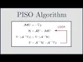
I've been getting a lot of requests recently to do a follow-up video on my simple algorithm video and actually take a look at the peizo algorithm because these two really are the main two pressure velocity coupling algorithms that you see and a lot of CFD codes and I'm really excited to bring this video to you actually because looking through the internet and the various sources I could find often the difference between the two algorithms is quite confusing it's not very clear what the real difference is between them beyond simple is often used for steady-state flows
and piezo algorithms often used for transient flows so what I've done here is I've really dug into the equations and actually managed to work out what the difference is in the loops between the equations and I'm really excited to bring this this video to you I really think are you going to enjoy it and finally really understand what the difference is between the two algorithms so yeah sit back take some notes it's quite a long video so we've got a lot of equations and background to go through but I know you're gonna find it extremely
useful so just to start things off with a background and a reminder of all of the pieces of the algorithm that you'll need to know and remember and then after we've been through the background I'll go in and look at the actual solution process that the algorithms use so just a reminder of where we start for an incompressible flow situation we have the continuity equation equation one and the momentum equations they're in equation two and for this simple system what we can see is that we've got four equations that's the continuity equation and three momentum
equations and we've got four unknowns pressure UX UI and you said four equations and four unknowns so that means we can find a solution however if we just look at those equations the first thing we noticed is that there's no equation for pressure so that's the first problem in the pressure velocity coupling problem now for a compressible flow we have an equation of state like the ideal gas law and we could use that to calculate pressure but for incompressible flow systems for example if we have water then we can't use that to calculate the pressure
and the second problem which we have here in the incompressible navier stokes system is that the continuity equation equation one is really a restriction on the velocity field that we compute so the way you should really think about this system is if you solve the momentum equations equation two you'll get a UX and UI and a you said and those components together have to satisfy the continuity equation to be a valid solution so you can't just take any solution of equation two the solution has to be specific and has to satisfy the continuity equation so
really for the incompressible system the continuity equation is a restriction on the solution that we compute and so this is what's often called the pressure velocity coupling problem and the PISA algorithm and the simple algorithm are two algorithms that we can use for incompressible flows to deal with this problem now when thinking about how we solve this problem the first thing we need to do is think of things in matrix form rather than in differential form which we saw that in the previous slide and the first step we can do is write the momentum equations
in general matrix form and you see that they're in equation three we've got a matrix of coefficients M multiplied by the unknown velocity back to you and then that's equal to negative of the pressure gradient there on the right hand side and how do we perform this discretization well we do that usually using the finite volume method and I've got other videos on this channel detailing the finite volume method or if you want to see things in more detail you can look at the various courses that I have available and that will show you how
to get that matrix of coefficients em there but generally when we're thinking of pressure velocity coupling problems we want to be thinking of things in matrix form so we've got mu is equal to minus the pressure gradient there on the right hand side and so that's a reminder of what those terms mean now it's also worth remembering that the matrix of coefficients M all of those coefficients are known and we calculate those and know what they are depending on what sort of discretization schemes we use for the convection term the diffusion term and so on
and I've got other videos on this channel how you discretize the individual terms but for now we want to be confident that we're just starting with that general matrix equation mu is equal to minus the pressure gradient there now at this stage in our pressure velocity coupling problem what we could do is take the pressure and the pressure gradient from the previous iteration or the initial condition and then we could just solve that equation directly so we know the matrix of coefficients m and we know the source term on the right hand side from our
initial guess or previous iteration and that would allow us to compute a velocity vector or the momentum field you now because this is the pressure velocity coupling problem it's worth noticing that when we solve that momentum equation the velocity vector U there does not satisfy the continuity equation as a reminder remember the vector u V and W has to satisfy the continuity equation for it to be a valid solution so at this stage when we solve the momentum equation this is often called a momentum predictor in the algorithm and it's a prediction because we've got
a guess for the velocity field and it doesn't currently satisfy the continuity equation now a small side note for those of you who use open foam and like to dive in and actually look at the equations in the source term in their source code you'll often see this momentum predictor stage written as you can see there at the bottom of the slide if clearly solving a momentum equation and that's equal to a source term which is the pressure gradient there on the right-hand side now when we're analyzing a look at the looking at these algorithms
there are a few other extra stages which we need to think about which will help us when we analyze the system and look at how the pressure velocity coupling algorithms are put together and the first stage in all of these is if we think of that matrix of coefficients M there what we can do is extract the diagonal from that matrix and the diagonal component of the M matrix is known and I'm going to use the notation a there than a matrix and you can see that it's just taking extracting those coefficients off the diagonal
and using that to make in matrix now if you follow along with the various sources in the literature you may see this written as a sub P instead of capital A which I'm using here I prefer to use capital A just as a reminder this is a matrix just like everything else whereas if we used an AP we could confuse that with the value so from the M matrix we can extract the diagonal if we want and what why would we do that what can we do with this a matrix well the thing to remember
is that with a diagonal matrix it's very easy to compute the inverse of the matrix and the matrix the inverse of a diagonal matrix is just 1 divided by the diagonal coefficients there which you can see in equation 7 and for those of you follow along the sources in the literature you will often see this written as 1 over a P again one of AP it's just the same as the inverse of this a matrix but I first call it the inverse because it's more correct and it reminds us what we're actually doing and again
if you follow along an open phone you'll often see this 1 over a P written as you can see there in an extract from the source code from sometimes called r ua which means the reciprocal of the a component there from the u equation so now that we've extracted the diagonal from the M matrix we can do a bit of manipulation and with that manipulation we'll see another matrix called the H matrix appear which will often see if you look through the sources in the literature so if we think back to our momentum predictor equation
which we have there in equation 8 instead of mu we're going to write that as au minus H now a as a reminder is that diagonal matrix that we extracted from the M matrix and then the H matrix which you can see there it's just the residual of all the stuff that we've got left so we extracted the diagonal and then all the stuff that's left but we're going to bundle that together and call that the H matrix so the reason I'm using H it may seem random at this point why is he choosing H
what does it mean well H is often the notation used by open foam and sources in the literature if you follow along so I'm deliberately using H here so that you know exact what it means now there's a small tripping point here which you could easily make mistake if you're not careful and that's notice that we're using the decomposition in equation 9 there so mu is going to be au minus H and not the decomposition which you can see there in equation 10 so what do I mean by that specifically well if you think of
the M matrix if you just took the M matrix and stripped out the diagonal then the remainder of that specific matrix you could call H now it'd be equation 10 there so that would be all of the off diagonal components and then zeros along the diagonal and that's specifically not what we're going to do there and the reason that we don't perform that decomposition equation 10 is we want to be able to rearrange this equation for you and that's going to be multiplying by the inverse of the a matrix there so if you thought about
multiplying equation 9 there by the inverse of the a matrix you could rearrange for you however if we used equation 10 and multiplied by the inverse of the a matrix we wouldn't be able to rearrange easily to get that u vector there so we've deliberately using equation 9 there for the decomposition and that's very important to remember but it's often skipped over if you look at a lot of the sources in the literature so this is just note of we are rearranging that M matrix the matrix of coefficients multiplied by the velocity vector that's going
to give us au minus H is the main decomposition here in the algorithm the rest follows relatively straightforwardly so you may want to take a few minutes just to go over that point in your heads so now that we've got that decomposition that's equation 11 mu we're going to replace by au minus H and we could just rearrange that to get things in terms of H and a reminder here that H is just the residual that we're getting after performing this decomposition and why do we care about the H matrix well the H matrix allows
us to calculate the source term for the pressure equation so we are going to use the H matrix don't worry if you've seen my video for the simple algorithm you will have seen this matrix appear for but I just wanted to line things up for you first to say where's this matrix coming from and what does it mean it's the residual that's left after we strip out those diagonal coefficients from the M matrix so as a reminder we've got the momentum predictor we've solved the momentum predictor to get some kind of velocity field and what
we now need to do is we need to have a way of calculating the pressure and the way we do that is by deriving a pressure equation then again if you've seen my video on the simple algorithm this is just repetition and you'll remember how this appears so if we start with equation 13 there that's we've got au minus H on the left hand side and then minus the pressure gradient on the right hand side that's the momentum equation as before and then the key step is to multiply by the inverse of the a matrix
as we showed before and of course the inverse of the a matrix is easy to calculate because it's diagonal and we multiply everything by the inverse of the a matrix we get an expression there in equation 14 for the velocity and you can see the velocity there is a inverse multiplied by that H matrix minus a inverse times the pressure gradient now just think about what we've done here all that we've done is rearrange the momentum equation to get to equation 14 and that's an expression for the velocity field but if we want to get
an equation for pressure what we can do is substitute equation 14 into the continuity equation so up until this point the continuity equation has just been a restriction on the velocity field that we compute so we've computed a velocity field and it would have to satisfy the continuity equation to be valid but now what we're doing is we're actually going to use the continuity equation to derive a new equation for pressure that we can solve instead so instead of having a restriction we now have an equation that we can solve from that's much easier so
if we substitute equation 14 into the continuity equation we arrive at equation 15 there and what you'll see straight away is that the unknown is the pressure there P on the left hand side we've got the laplacian or nablus squared of depression of the pressure and them on the right hand side we've got a source term which is a inverse multiplied by the H matrix so this is just a reminder this is all background so far for setting up these algorithms we've got a momentum predictor that we can use to calculate a velocity field and
now we've also got an equation for pressure and using those together we can come up with an algorithm for solving the momentum and pressure equations together while ensuring that the velocity field satisfies the continuity equation so now I've got this pressure equation I just want to highlight for you for a few of you who might be following along either using sources in the literature or by actually digging through the open foam or other CFD code you'll see this pressure equation sometimes written as you'll see there in equation 16 we've got 1 over a P instead
of the inverse of the a matrix and the same thing and some people use H of U instead of just H as it is to calculate that residual matrix on the right hand side I personally just prefer to use H because I feel like with the extra u it can get confusing there and in open foam you'll often see the fragments scattered through the code at various places looking like this we've got that first expression for the inverse of the a matrix the second expression there is an expression for the H matrix multiplied by the
inverse of the a matrix and then right at the bottom there you can see an expression for the laplacian of the pressure so that's the pressure equation that we would be solving and on the right hand side you've got a divergence term for the H by a term on the right hand side so if you're looking through the source code or various sources in the literature when you see these things recognized as a or H or laplacian of the pressure gradient you'll understand now where they're coming from and you can follow the derivation that I've
just given there if you want to derive it for yourself but now let's actually go ahead and look at the algorithms so you can see how the simple and pizzo algorithms actually solve the system together and what I'm going to do is call these pressure velocity coupling algorithms because they're specific for incompressible flows when we have a pressure velocity coupling problem so in the algorithms the first thing that we always do is solve the momentum predictor first and that's equation 17 we know the matrix of coefficients m and we have an initial guess or the
previous iteration of the pressure term on the right hand side and we solve that for the velocity field and the velocity field is a guess as before the reason it's a guess or it's a prediction is because it doesn't yet satisfy the continuity equation but now that we have the velocity field you a guess we can calculate the H matrix that's equation 18 so we can see there on the right hand side the H matrix actually depends on the velocity field and we've got the a matrix there which we strip out from the M matrix
so momentum predictor first and then we jump straight in to calculate the H matrix and the reason we calculate the H matrix is because the H matrix is a source term on the right hand side of the pressure equation and that step I think is sometimes missed out by some of the explanations which you may see on the Internet so now we can solve the pressure equation and on the right hand side there you can see the H matrix which you've just calculated and the inverse of the a matrix which we stripped out from the
M matrix and solving equation 19 gets us the pressure field and once we have the pressure field we can then use equation 20 to compute a new velocity field now the difference here when we calculate the velocity field is that the velocity field here is calculated explicitly we're not solving the matrix equation we're calculating it directly from the a matrix the H matrix and the new pressure matrix which we just calculated there an equation 19 and this is called an explicit pressure correction and what it means is the velocity field that we compute here will
satisfy the continuity equation so it's you might say it's solid a solenoidal vector field but it satisfies the continuity equation and this is exactly what we want this is the corrected velocity field at the end of the algorithm and for some of your interests this is why for example the simple algorithm is called the semi implicit method the semi implicit means that it's partly explicit and the explicit part is equation 20 there where you're explicitly calculating the velocity field directly from the pressure field that you've just calculated however there's a small problem here and that
is if we think back to the pressure equation equation 21 on the right hand side the source term has got the H matrix in there and what we know is that the H matrix depends on the velocity field U which you can see there in equation 22 now originally we use the momentum predictor to calculate that H matrix but now what we've done is we've corrected the velocity field so U is different now to what it was before and of course what that means is that if u is different H is different so the source
term in the pressure equation their equation 21 has changed so what that means is is that the pressure field is no longer correct and even though our velocity field satisfies the continuity equation our pressure field is not correct and it needs updating and maybe take a few minutes to think that over and if you just write the equations out for yourself you'll see that actually the pressure equation is no longer correct and we need some way of updating this H matrix so that we can re solve the pressure equation and this is the key point
to where the simple and the piezo algorithms come in and this is often not explained very well on the internet and in other sources where people talk about relaxation factors and time steps and things we often get confused but really this is the key step it's how do we go back and update the pressure equation by updating that H matrix there and the two algorithms are really two different methods of updating the H matrix and I'm going to start with a simple algorithm because it's easier and then I'll show you the Pizzo algorithm after which
is a different way of updating the H matrix and the pressure equation so the simple algorithm is very direct and what it says is well we need to update the H matrix so I'll just go all the way to the start and sold the momentum predictor again and so I just go back through the entire loop and for those of you who might be finding that difficult to follow in your heads like I was I find it much easier to actually just write down the equations and just look at them and see where are we
updating so reminder of what the loop will look like for the simple algorithm we start with equation 23 we solve the momentum predictor once we have you the velocity field we calculate H which is equation 24 then we calculate the pressure field by solving the pressure equation there and in 25 and then we update the velocity field there in equation 26 but now what we do to correct the H matrix is go all the way back to the start of the loop equation 23 solve the momentum predicts it again and use that to update the
H matrix so that we can then solve the pressure equation again and it's worth noting sometimes when you look through these algorithms that this loop is often called an outer corrector loop and the reason it's an outer corrector loop is with the simple algorithm we're going all the way back to the start of the process and solving the momentum momentum predictor again so really it's a very direct way of doing things the user is quite a long loop the piece of algorithm is slightly different which we'll see in a minute but hopefully by writing those
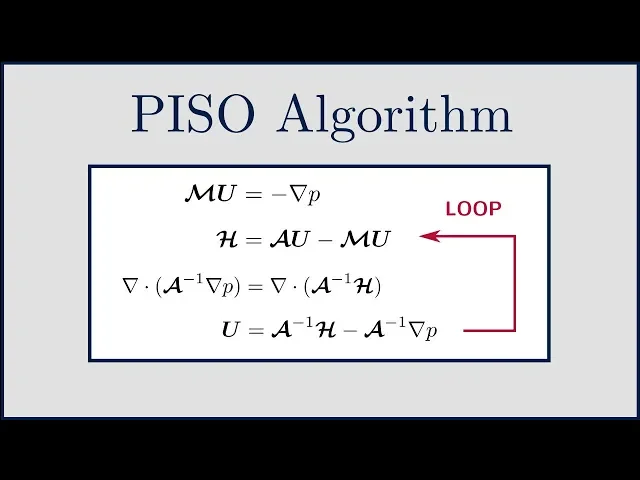
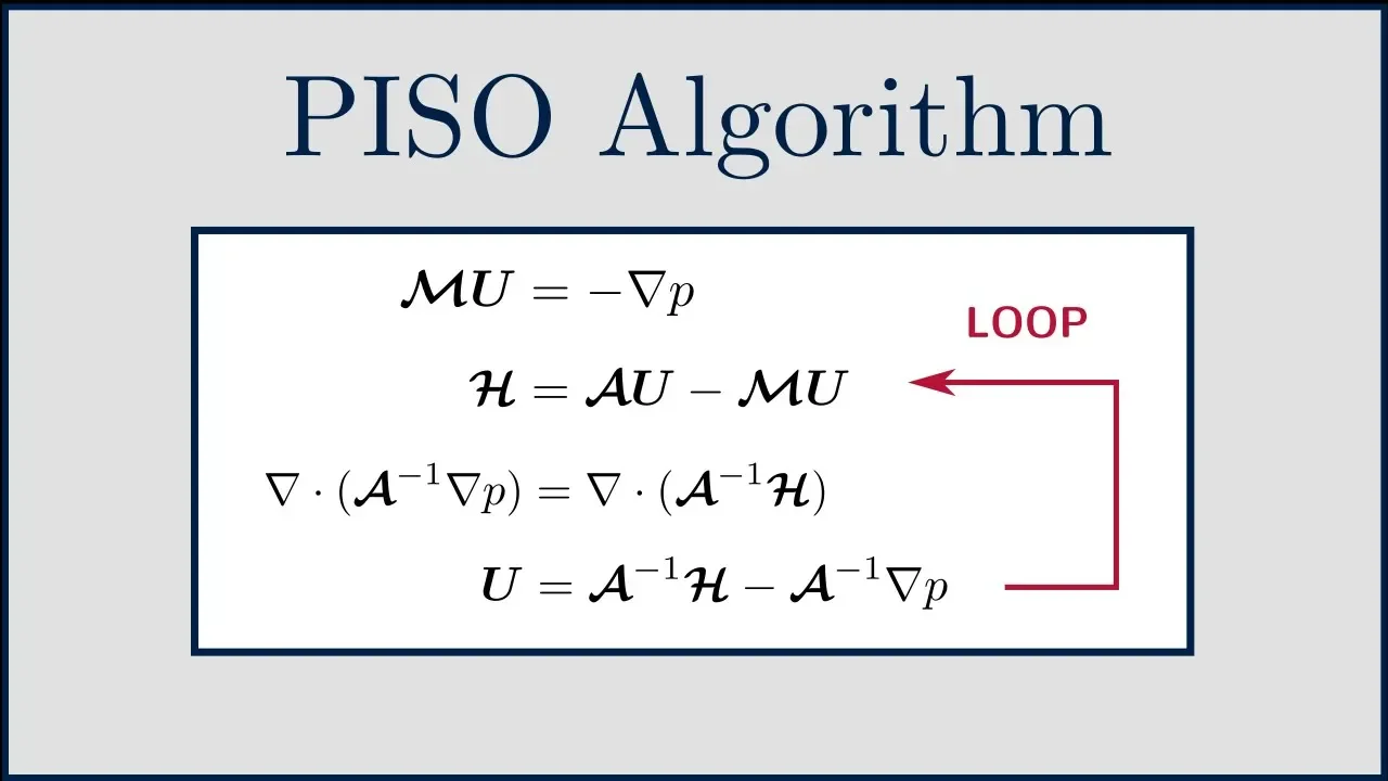
equations down you can really see exactly where the loop is in the simple algorithm and it's worth noting so far that I haven't said anything about time stepping or relaxation or convergence or anything this is just the stages and the equations that you would solve if you were using the simple algorithm for your pressure velocity coupling so what about the PISA algorithm well in the PISA algorithm what we do is we solved the momentum predictor once so we start with the equation 27 and solve that once directly but then what we do as before we
calculate the H matrix and use that to solve the pressure equation equation 29 and then once the pressure equation has been solved we correct the velocity field there using equation 30 but the difference between the peizo algorithm and the simple algorithm is that rather than going all the way back to the start there and solving equation 27 which arm straight to equation 28 so you can see equation 28 there to complete the a matrix we need a velocity field and rather than use the velocity field the map from the momentum predictor we're going to use
the velocity field directly from the one that was just corrected there in equation 30 and so you can see that actually now we're looping over equation 28 29 and 30 and we only solved the momentum predictor once so this loop is a lot tighter or any looping over three equations and this process is often called an inner loop if you look at CFD manuals and in source codes so actually at a fundamental level the difference between the piece of algorithm and the simple algorithm is very slight and it's just which way we're updating the loop
there now it's worth now that we've looked at what the difference is between the two algorithms in the order that the equations are solved now what I'm going to do is introduce some of the other concepts and reasons why you might choose to use a simple coupling or a piezo coupling depending on your simulation now the first place to start is really to think historically about these algorithms and where they came from and what they're originally proposed for walkers that will usually help you to decide which one you'd like to use and the simple algorithm
was proposed first in the 1970s and the simple algorithm was originally intended for steady-state flows now originally intended doesn't necessarily mean you have to use it for a steady-state flow but it was originally intended for steady-state flows and just a reminder with steady-state flows what that means is we don't have a time derivative so that expression you can see there an equation 31 that D UDT does not exist for a steady-state flow and what does this mean for the equations that we're solving well if we think about a transient flow where we have a very
small time step then if you look on the right-hand side of equation 31 the U P divided by delta T is going to get very big as the time step gets very small U P over delta T gets very large so if we think of this in terms of the overall May Tracie's that we're constructing the D UDT term gets a lot bigger as our time step gets a lot smaller and what that means is if we think of all of the terms in the equation we have time derivatives we have convection diffusion gravity forces
and source terms then the time derivative that is becoming dominant it's becoming a lot larger than the other terms and what you'll see there if you look is that we've got a u sub P and that usually in CFD terms means that the term is on the diagonal of the matrix so the U P over Delta t occupies the diagonal of that M matrix and as delta T gets very small that means the diagonal of the matrix gets very big and for those of you who think back to your linear algebra or look on the
internet for general concepts in linear algebra as the diagonal of that matrix gets a lot bigger the system tends to get more diagonally dominant and that's the phrase that's often use what it means in practice is that the equations get more stable they're easier to solve they take less iterations to solve and so what does that mean it means generally for a transient flow the matrices that we construct are more stable and take less iterations to solve and are less likely to diverge and the simple algorithm was not intended for these flows the simple algorithm
was intended for cases where the matrices don't have the time derivative and they're more likely to be unstable and what the simple algorithm does in those instances is we use under relaxation and in this instance under relaxation is used to artificially increase the size of that diagonal term because we don't have a dutt we need to make something else instead so that we can inflate that diagonal on the matrix to make it more stable so if you were just thinking about this intuitively you may think that a transient flow would be easier to solve than
a steady-state flow but actually steady-state flows to him to be a lot more unstable it's just that transient flows take many more iterations to solve because of the time stepping so it's a bit counter and so in the simple algorithm and the when it was originally proposed under relaxation is often employed and so if you use the simple algorithm yourself you will often see under relaxation in the equations whereas you may not see them if you've got a transient flow now this under relaxation is slightly different to a traditional under relaxation which you may be
used to from general algorithms and the way I'm going to explain this to you is by starting with equation 232 there and you can see you've got a PU P that's going to be the diagonal terms in the matrix and then you've got the off diagonal terms in the summation there a and um is equal to a right hand side matrix so an equation 32 is basically just a general form of a linear algebra the matrix equation there and when we apply under relaxation to the momentum equations what we're going to do is add in
two additional terms there and you can see these terms in red in equation 33 we've got a 1 minus alpha over alpha multiplied by AP u P so the AP u P is going to sit on the diagonal of the matrix and alpha is going to be the under relaxation factor which is always between 0 & 1 and what we've done is we've added that term to the left and the right hand sides on the left hand side we've got the current value but on the right hand side we've got the old value of the
velocity field and the reason we can add this to both sides of the equation is that when the equations are converged you old will equal you new and these red terms will cancel out and disappear but until we get to that point those terms are going to be different and they're actually going to help us to converge the matrices so if we look at the left hand side of equation 33 we can actually group those first two terms together and then we arrive at equation 34 and you can see that the equation that's got an
under bracket there is now scaled by 1 over alpha and that is the diagonal of the M matrix so ap again being those diagonal terms but they're mount applied by 1 over alpha and because alpha is between 0 & 1 if we make alpha a lot smaller we're going to artificially inflate that diagonal and make the diagram a lot bigger in in comparison with the other terms and that's typically what we would get with time stepping so we can see that this is totally artificial we've just manipulated that diagonal to make it bigger and this
will make the equations more stable when we're solving them in a steady state form so this is the premise of under relaxation that the simple algorithm typically uses and it's worth comparing this with the traditional way to do under relaxation where if we had a value that we calculated in an algorithm we could update that using something like equation 35 where we add on a fraction of the new value to the old value when updating the field and this form of under relaxing the fields so pressure turbulent kinetic energy temperature is often applied to pressure
turbulent kinetic energy and temperature but the matrices themselves are under relaxed in the momentum equations and to be honest I'm not too clear with why that that process happens it's not very clear from reading through the literature however for you when you go through and if you look at it be aware that there are actually two different types of relaxation one different type that's applied to the momentum equations that's increasing the strength of the diagonal there and that we've also got direct relaxation of the fields pressure turbulent kinetic energy and temperature so this under relaxation
is typically applied to the in the simple algorithm however the piezo algorithm is different now the piezo algorithm was introduced slightly later than the simple algorithm historically it was introduced in about 1986 and it was originally intended for unsteady incompressible flows so again for the unsteady flows we do have a time derivative so that diagonal in the matrix the M matrix there is a lot larger and the system is more diagonally dominant so we don't actually need under relaxation on the condition that our time step is very small so if we have a very small
time step and our current number is less than one we can actually get a way without any under relaxation at all and this is how the PSO algorithm was originally proposed so if you look through any source code on Pisa algorithm and piezo loops you'll often not find any under relaxation at all and that's because it's assumed that the current number is very small and we using very small time steps now why why was the piece of algorithm introduced and what was it for why couldn't we just use the simple algorithm you know we could
take our first time step and fully converge that time step using the simple algorithm and then just step on to the next time step well if we think about it then actually with the simple algorithm we often need a lot of iterations to fully converge when we apply it and common practice tends to be we need a few thousand iterations often five thousand to fully converge a steady-state flow with the simple algorithm but if we have an unsteady flow we're gonna have to do a lot of time steps and so doing five thousand iterations every
time step tends to be really inefficient and we often won't be able to get a full solution and so the PISA algorithm is deliberately a lot shorter than the simple algorithm we do one momentum predictor and then too often two inner loops of the pressure corrector there and that's often fairly sufficient to converge the time steps after we've proceeded over the initial transient in our simulation so this is why the PISA algorithm was introduced it was introduced after the simple algorithm and the reason for it was we can't afford to do 5,000 iterations of the
simple algorithm every time step we need something that's shorter and quicker and will allow us to rapidly push through the time steps now there are of course more modern pressure velocity coupling algorithms which you may have heard of and some of these will tend to try and do even better than the simple and piso algorithms so one such example would be the pimple algorithm which you may have heard of an open foam where you can actually use larger time steps and then converge the time steps partially maybe doing 15 or 20 iterations within a time
step but allowing you to extend the current number greater than one but I'm not really going to look at those algorithms here I just wanted to focus on the simple and piso algorithms now one thing I want to finally touch on before finishing it are the non orthogonal characters because if you're looking through the source code you may see these characters as well and it's useful to know what the difference is between an inner character and outer character on a non orthogonal corrector so when understanding non orthogonal characters the first thing to do is to
look at the pressure equation which you can see that in equation 38 now notice that the pressure equation is essentially a laplacian or more technically a Poisson type equation where you've got nablus squared times the pressure is equal to some source term on the right hand side and of course if the mesh is not orthogonal that means this equation needs to be solved several times in a row updating the source time each time to account for the non orthogonality and for those of you who haven't come across this before it's worth going and looking at
my video on non orthogonal correctors to understand why this is needed for meshes that aren't perfect squares so as soon as the mesh is not perfect squares you have to include normal Fogle and correctors or at least consider them if you're going to get an accurate answer and so how do these non orthogonal characters appear in these simple or piso algorithm when we're thinking about it well what we do is that we iterate the pressure equation directly in a row with the number of non orthogonal characters that we want to use now at the moment
this might be a bit overwhelming for you my thing this there's a lot of equations going on and I can't quite remember which equation comes where and how many times do I need to loop it so what I've done here is I'm just gonna go through a quick example of what the sequence of equations will look like if you have non orthogonal characters in a simple algorithm and normal fokin or characters in a Pizzo algorithm so you can actually see them start to think through are which equations are being solved and when now the first
example here is a simple algorithm and in this instance we're going to have two non orthogonal correctors and just a reminder of how the algorithm works we start with the momentum predictor their equation 39 and once we've solved that we calculate the H matrix as normal there in equation 40 and what we would then do now that we've got the H matrix is we can get the right-hand side of the pressure equation there an equation 41 we've got H and we've got the inverse of the a matrix so we can solve the pressure equation but
now because we are doing orthogonal orthogonal characters we continue to solve that pressure equation immediately so in this instance we have two non orthogonal characters so we end up solving the pressure equation three times in a in a row there 41 42 and 43 and once we've done the non orthogonal correctors we then go on to proceed with the algorithm as we normally would so for simple we would correct the velocity field there using equation 44 so it satisfies the continuity equation and then because this is the simple algorithm we use all the way back
to the start there and go back to equation 39 and we would continue to loop through these equations until we were converged so if you took out equation 42 and 43 that would just be the normal simple algorithm all that we're doing with the normal thug little characters is just directly solving the pressure equation again immediately with an updated source term to account for the non orthogonality so what about the peas our algorithm very similar the first thing we'll do is we solve the momentum predictor equation 45 now remember with the PISA algorithm we only
solve the momentum predictor once in each loop so then what we do is we dive into the inner loop and we calculate the H matrix once we've got H we can solve the pressure equation there equation 47 as we have the right-hand side now with two non orthogonal characters we would just repeat the pressure equation again immediately and go equation 48 49 those are our two normal Thorin and Coretta loops and then we can finally correct the velocity field there in equation 50 once we have that we can use it to update the H matrix
and then again go back into that pressure equation because remember with the Pizzo algorithm we use the corrected velocity field their equation 50 to update the H matrix rather than the momentum predictor which is what we would do if we were using the simple algorithm so hopefully just through those last two examples it might be a bit easier for you to follow of which equation am i solving in what order and what's the difference between the Pizzo and the simple loops in the process that we use to solve them so just wrapping up with a
summary of what we talked about here and a few reminder points for you all pressure velocity coupling algorithms whether that's piezo is simple or another one which you may see in the literature will solve a momentum predictor first so you'll be solving mu is equal to minus the pressure gradient all of the algorithms will solve that and then what we'll do is we'll move on to solve a plus on equation for pressure and use that solution to update the velocity field so that it satisfies the continuity restriction now at this point what we need to
do is update the source term in the pressure equation and solve it again and the difference between the simple and the piso algorithms comes into how we update the source term that h matrix we either do that by looping all the way back to the start and solving the simple algorithm again or by going directly back and using the momentum field that was just corrected to satisfy the continuity equation so there it is that's the end of the video I hope you guys enjoyed that and found it as useful as I did going through it
it's really useful to actually finally see what the difference is in the loops between the two algorithms so let me know what you think did you enjoy the video did you find it useful I know it was getting a lot of requests to do a video on the PISA algorithm and let me go let me know in the comment section below what you guys thought are there any other really pressing videos that you think I should have a go at because there are still many different areas of CFD which aren't covered at all well and
I'm slowly trying to get through the big topics one by one so that we can finally build up a picture of how all the aspects of the modern CFD codes finally work so thanks a lot for your support again guys and I'll see you soon