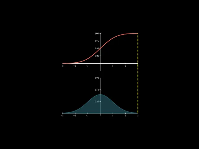
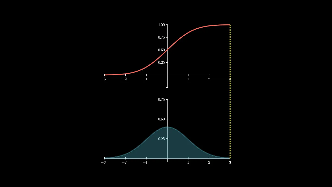
foreign we are going to plot these two functions more specifically the normal distributions PDF and CDF function and we are going to create this nice animation where we are projecting the area of the probability density function on the bottom so it's a cumulative density function on the top and we're going to drop both of those plots simultaneously let's get started first thing we're going to do is we're going to import all dependencies from mannum I'm going to also use the normal distribution set of functions from this stats package in scipy I'm also going to bring an OS to run the command on the op on the operating system level I'm going to take the scene I'm going to extend it and make this a projected area scene and the construct function is what we Implement to construct all of our scene animations I'm going to declare my mean and standard deviation to be 1 and I'm going to declare the lower and upper bounds of the plots for the top and bottom one the PDF and the CDF and they're going to be within three standard deviations so that's the lower and upper bound the value tracker again this is a very important piece of functionality in mannum that allows you to interpolate a bunch of values between animations using a single floating point value that this wrap around that this wraps around I'm going to clear my axes and oh and I'm going to declare the value tracker to start at the lower bound the axes are going to for the X range are going to fall in that X lower f x up or I defined earlier and it's going to have ticker tick increments of one the Y range is going to range from negative 0. 05 to 0. 75 and then 0.
25 and again this axis is for the probability density function the PDF that's the bottom plot with the bell curve and I'm not going to show the arrow tips and I'm going to configure this to include the numbers the CDF that is the s-shaped curve that captures the area of the PDF that is going to use the same range as the PDF from the X lower to X upper plus or minus three standard deviations around the mean with a tick increment of one and the Y range is going to show a full probability between 0 and 1. I'm also going to put a little bit of buffer of negative 0. 25 below it so it so that the screen doesn't hug the x-axis and I'm going to use 0.
25 increments you'll you'll notice that I the way I chose those y ranges just really depends on how much of the plot you anticipate will fall within the given y range so obviously if you make the Y range too wide you're not going to see the bell curve nor are you going to see the CDF and I know for the fact that the CDF is not going to exceed 1. 0 because it's probability I'm not going to show the tips and I'm going to include numbers but I'm going to exclude that negative number I don't want to show that on the axis and then um so negative 0. 25 any numbers with negative 0.
25 which is on the Y range those are not going to be included and this applies to both taxis although I could have targeted the y-axis specifically don't have to though now I'm going to take the those two axes put them in a vector group a v group and then I'm going to arrange them upwards so it's going to show the PDF on the bottom the CDF on the top I could have done it down and flipped these that would have achieved the same result then the buff this is the number of units to put a buffer between those two axes then I'm going to scale to fit the height of 6 units so I believe that that Mana by default has eight units high on the screen so we're just going to use six of those and we'll scale it keeping proportion using the scale to fit height function both the PDF and the CDF axes now I'm going to declare the PDF function plot and its area so I'm going to always redraw plotting the PDF function passing the given x value and the mean and standard deviation all of that to the plot function I'm only going to plot the curve up to the value tracker's X values so I call Value trackers get value function which again we declared all the way up here and it's only going to draw the upper Bound for the plot based on what the value tracker currently is when we set that animation this is going to create that nice effect of of writing that plot left to right it's also going to be blue and by doing the always redraw it's going to always redraw this plot on every single frame then I'm going to plot the the PDF function in full right here just as a reference I'm not going to actually use it and I'll explain I'll explain what I what I use it for next the reason why I want to include it is because I also need to get the area of I need to get the area up to a given a given plot value so I need to have access to the full plot even if I'm not displaying it just to get the area up to a given x value and then the range is going to be uh from the lower to the again the value tracker's upper upper function and this is going to plot the area uh for the PDF up to this value the CDF is going to is going to always withdraw in a very similar way as the PDF partial plot so the CDF partial plot pretty much follows the same pattern drawing that s-shaped curve um but using the CDF function to calculate the cumulative density function for that given x mean and standard deviation now that projecting dashed line that connects these two graphs I am going to again always redraw it because the value tracker is going to steer steer this in between each frame and animate it I'm going to call dashed line it's color is going to be yellow the star is going to be the value trackers given value the value tracker is given value up to zero now here's here's the here's the thing though is that this line is connecting two plots outside of their axis reference system so I need to convert those axis coordinates uh for the for the start and end of the line for the PDF and the CDF respectively and I'm going to call their coordinate to point functions to convert the the the given x value that we're tracking and make the Y zero so it's always going to connect it to the bottom the bottom of the x-axis at the x-axis and it's going to end at the cdfs the cdfs the cdf's x x value and the probability values so the the Y value on the CDF and that's what this is doing right here so I'm passing the value trackers get value to the cumulative density function and passing at the mean of standard deviation as well so I probably should emphasize one more time that the axes c2p function that converts a coordinate on an axis to a coordinate on the screen and by doing that we are able to get these two axes to talk to each other and connect a line between them so this is one of the most powerful features in manum in my opinion is this ability to take relative systems based on axis to a point system on the entire screen and this is going to be this is going to produce that nice dashed line between uh the PDF and the CDF uh connecting those two graphs and then finally I'm going to add the axes those partial area plots even though there's no volume in them yet or there's there's no substance to them yet because the value tracker is at zero so the Min and Max of X are at zero and then the projecting line is going to be all the way on the left side as well and that's going to be a starting position I'm going to wait one second and then I'm going to Simply animate by calling value trackers animate functions and then set value and set it to the xopper which is going to be the three Stan which I declared all the way at the beginning up here which is going to be mean plus three times standard deviations that's the max of the X range and I'm going to do that for seven seconds and then I'm going to wait one more second finally I execute the command for manum so I could do this in Windows or Mac OS or Linux terminal but I'm just calling this straight from python using the OS and just checking if this is the main calling the manam use it use a 4K quality and I'm going to suppress warnings I'm going to play the the result immediately disable caching I'm going to Output to the projected area scene this actually should be an mp4 and then I'm going to call this file right here the scratchpad.