Last time we talked about one of the analytic study designs called a case control study. another feature of the analytic study design is to measure the relationship between disease and exposure. So in a case control study, the strength of the relationship between exposure and disease is quantified and compared using the odds ratio.
So odds here is defined as the ratio of the number of people with the disease of interest to the number of people without. Remember that the odds is not probability because this is a ratio not a proportion so it can go over 1. Now given an exposure, there will be two odds, one for the exposed and the other for the not exposed group.
So you take the ratio of these two odds then it will become the odds ratio which is the ratio of the odds of having a disease given an exposure to the odds of having the disease without the exposure. So here is the step-by-step procedure to calculate an odds ratio. First, you need to identify the number of cases with disease and healthy controls.
Once you do that, then you need to further split the cases and controls based on their exposure status to a risk factor of interest. So the table shown here is what's called a 2x2 contingency table. Here the columns represent the disease of the study sample and the rows represent the exposure status of the study sample.
So here A represents the number of cases who are exposed to a certain risk factor under investigation whereas B represents the number of healthy controls exposed to the same risk factor and the C represents the number of cases who are not exposed to the risk factor and finally the D is the number of the healthy controls (that) were not exposed to the risk factor. Now you may be wondering how you don't get disease when exposed to the same risk factor to which the cases are exposed. Conversely, how come you get disease when not exposed to exposed to the risk factor?
In fact, I told you about this before. There's rarely a single, definitive cause behind a disease. It is not one to one match relationship.
Disease results from multiple risk factors and their interactions. So not all the cases are necessarily exposed to the same risk factor. By the same token, some people don't get sick even after they're exposed to the risk factor because of the individual differences in resilience or other factors.
Therefore, the disease occurrence is inherently probabilistic interplay between different risk factors. So from this, we should estimate the risk with a given exposure for these four different possibilities to determine how more likely it is to catch the disease when exposed to a certain risk factor against when not exposed. Now you have to calculate the odds of having the disease for the exposed and the unexposed.
So the odds of having disease when exposed is A over B. So this is the ratio of the cases to the healthy controls when they are exposed to the same risk factor. And what is the odds of the unexposed group?
The odds of having the disease is C over D. Now the odds ratio is the ratio between these two odds. So it's the odds of having the disease when exposed over odds of having the disease when not exposed.
So it's A over B over B over D. So you multiply these two and that goes to denominator BC and multiply these two AD so this is the odds ratio AD over BC. Now this odds ratio is subject to NHST where the null is saying that odds ratio is equal to 1 or not statistically different from 1 which is saying there is no difference in the odds of having disease between the exposed group and the unexposed group.
On the other hand, the alternative is to say that the odds ratio is statistically different from 1 in two-tailed fashion. So in a nutshell, the idea is basically same as the t-test where. .
. so say if you take the log of OR, so that is actually log of AD over BC and by the rule if you still remember AD minus log BC and when log of 1 is zero. So that is a null basically we're testing the difference but when these two quantities are the same the difference will become 0 and the ratio will become 1.
So this is basically in the same form. So let's just take an example from here. Let's just erase and take a simple example.
So for example, if the odds of having an AMD, so AMD+ so you have AMD and AMD- so this is without and the exposure here is a smoking. So smoker+ means that you are a smoker and smoker- means you're not a smoker. Typically, it is thought that smoking is a risk factor to AMD.
Just hypothetically if the odds of having an AMD for being a smoker is 5 and the odds of having the same disease for non-smoker is 5. Then there is no difference in the odds. So smoking is not a risk factor to AMD.
So in this case, AMD (? ) that's a b c d. So the odds of having AMD when you're smoker.
So the odds smoking and so this is the odds of having disease when you're smoking. it's 50 over 10, which is B and then odds of having AMD when you're not smoking is 50 over 10 again. So the odds ratio is 50 over 10, 50 over 10.
So basically we have just same odds up and down. So that is 1. So in this case and smoking is not a risk factor because regardless of smoking and the odds of having the AMD is basically the same.
So in this case you cannot say that smoking is a risk factor. On the other hand, we have different odds now. So if the odds of having AMD for being a smoker is 5.
So the odds smoking is again to this 50 over 10 but odds of non smoke is now 10 over 10, which is 1. Now odds ratio is basically 5 over 1. So now the odds of having AMD is whooping five times that of the non-smokers, odds of having the AMD when you're not a smoker.
So in this case we can say that smoking is a definitely risk factor, well not definitely you don't know yet because you don't know how much the odds ratio should be bigger than 1 to say that this is statistically significant. So that is the question how big should be the odds ratio to say that is statistically greater than 1. So is the odds ratio of 5 statistically over and beyond 1?
So that is the question. So how do we determine the statistical significance of OR? You either compute P-value of observing the sample odds ratio or calculate the 95% confidence interval of the odds ratio to see if the interval includes no difference point which in this case of odds ratio is 1.
Typically 95% confidence interval is somehow more frequently reported than the P-value and the idea of how to make the statistical decision is very similar to how to read 95% confidence interval of mean difference in case of t statistics. So if the 95% confidence interval contains zero representing the zero difference, that means the mean difference is not statistically different from zero. It is only when both limits are negative or positive when the mean difference is statistically different from zero.
Likewise if the 95% confidence interval of odds ratio does not include 1, in this case one represents no difference, that means odds ratio is statistically significant. On the other hand, if the 95% confidence of confidence interval of the odds ratio contains or includes 1 in the interval that means the risk factor is not statistically significant in increasing the odds of having the disease. That's what it means.
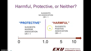
Again the direction matters. So if both limits of the confidence interval of the odds ratio are greater than 1 then that means the exposure is harmful like in smoking case whereas the exposure is beneficial when both limits are less than 1 say like taking Lutein against AMD. So the direction matters from one, from no difference point if it is greater than 1 then it is harmful if it is less than 1 it is beneficial.
So statistical representation of odd ratio is basically the same as the confidence interval of the mean difference or the mean, sample mean. Eeven though this equation looks complicated but it is not. It's really the same as the 95% percent confidence interval of the mean.
So the confidence interval is the OR, sample odds ratio plus minus the confidence coefficient. So if it is 95 then it's a 1. 96, 2, plus minus 2 standard error of the odds ratio.
That's all there is to it. And the confidence coefficient is exactly the same as the mean, sample mean confidence interval. But in calculating the 95% confidence interval for odds ratio and the risk ratio or the relative risk is a bit convoluted compared to calculating the 95% confidence interval for the mean.
So these are the steps in calculating the 95% confidence interval of odds ratio. So let's just take a look at each step we're using a worked example. So this is the actual data taken from the previous the Acanthamoeba Keratitis investigation.
So you're given the 2x2 contingency table, each cell filled with the number of cases and non-cases when exposed to the multi-purpose solution or not exposed to that solution. So first you need to calculate and the odds ratio. So odds ratio will become so that's 80 40 times 125 and 15 times 32 so we need a calculator okay so 40 125 okay so it's about 10.
42. So now we calculated the odds ratio. So what that means is that once you're exposed to that multi-purpose solution, so if you use that multi-purpose solution to clean your lens, then you have 10 times more likely to catch keratitis compared to who did not use the multi-purpose solution.
So once you calculate this odds ratio, you need to take the natural log of that odds ratio. So this is the results. So let's just.
. . So we have this value and.
. . see the ln, so that is for the natural log.
So you just click and you get that. 2. 3434 and so on.
So that's what we have. Once you have that, then you need to use this equation. This is simple.
You just basically plug in each number from each cell to this equation to calculate the standard error of the natural logged odd ratio. So that's how you calculate this and so let's just plug in those numbers using the calculator again. So we have 1 over 40 plus 1 over 15.
plus 1 over 32 and 25 equals this and you take the square root of it, you get that, 0. 3618. That is the standard of log odds ratio.
So now the 95% percent confidence interval in log space. We're still in log space. .
. a natural log odds ratio plus minus 1. 96 times standard error of the natural logged odds ratio.
So this is what we have (been) obtained. So if you do that, the lower limit is 1. 6342 and the upper limit is 3.
0526 which is still in the log space. So you need to do the exponentiation on these both limits to put them back into the real space (I meant in original scale). You just take the exponentiation of these limits, then you will get these values.
So in the actual log space (? ) so the real space you have lower limit of 5. 1254 and upper limit 21.
1703 so the actual odds ratio was 10. 42 and then 95% confidence interval is 5. 13 and 21.
17 and we know that this odds ratio should be placed in somewhere in the middle of this 95% confidence interval. So let's just look at if these numbers are actually the right numbers. e to the lower limit 1.
632. That's 5. 12.
That's 21. 1703. So those numbers are correct.
Now we know that confidence interval, 95% confidence interval for this odds ratio are these two. And this is how you interpret the 95% confidence interval of odds ratio so when you report you need to state the conclusion in the original scale not in the log scale. And you would just say something like the odds ratio for keratitis for the specific multi-purpose solution compared to the non-use of the solution or different brand is 10.
42, indicating the increased odds of keratitis for the people who use that specific solution and the 95% confidence interval of the odds ratio 5. 13 21. 17 indicates that the odds of having keratitis are significantly higher for the group exposed to the specific brand of the multi-purpose solution compared to the group without exposure because the confidence interval does not contain 1.
So this is what I have been saying already. So an odds ratio close to 1 indicates no associations between exposure and the disease and if the 95% confidence interval of the odds ratio does not include 1 then the result indicates a statistical significant association between the exposure and the disease and if both limits of the confidence interval are greater than 1, then the effect of the exposures are harmful whereas both limits of competence interval is less than one then the effect of the exposure is beneficial. Now here are the pros and cons of case-control study so the good things about case control study is that the study can provide stronger evidence than a cross-sectional study and that is coming from the calculation of odds ratio.
And it is a relatively efficient in time and cost because you don't have to wait until the disease occurs because the the case control study starts its investigation from the disease end after everything is said and done now you start the investigation. So it is relatively quick and you don't have to spend a lot of money on this and also it's easier to study multiple exposures and their interactions related to a specific disease. As we have seen, once you have disease and there are a list of possible exposures that may have been related to the disease.
So it's easier to study multiple exposures per disease but not the other way around. You cannot investigate multiple diseases given an exposure with case control study. And finally case control study is kind of ideal to study rare disease because the disease are rare, it is always the case that you do not have enough cases to have meaningful statistics or whatnot but the case control study starts its investigation from the disease end.
So by the time you start to run case control study, you probably have already enough cases to proceed with the case control study. So case control study is suitable to study rare diseases and there are some other not so good things about case control study and the first one is case control studies are still limited in deciding causal relationship between disease and exposure. That's because you still cannot establish this temporality between the exposure and disease because case control study collect the data after disease has already occurred and then you're just going backward in time to find out the cause so still the case control study is missing the temporality.
And this was discussed already. It is in the most time consuming part to match the case with control group. So the control group should be more or less comparable in every aspect to the case group except for that they don't have the disease.
And sometimes it gets really difficult to select a matching control group and case control study is also subject to bias such as selection or recall bias. Here bias refers to any systematic error in any type of epidemiological study that result in an incorrect estimation of the association between exposures and outcomes. So investigator can introduce bias into a study as a result of the procedures for identifying and enrolling subjects or from the procedures for collecting or analysing information.
Therefore it is important for investigators to be mindful of potential biases in order to reduce their likelihood as much as possible when they are designing a study, at design stage because once bias has been introduced then it cannot be removed at the analysis stage. Briefly, a selection bias can result when the selection of subjects into a study or the likelihood of being selected in the study leads to a result that is different from what you would have gotten if you had enrolled the entire target population. On the other hand, recall bias occurs when there are systematic differences in the way subjects remember or report exposures or outcomes which is typical in case control studies.
For example, subjects with disease may remember past exposures differently than those who do not have the disease. So these are the things that the case control study is good for or not so good for.