Hello everyone, Today I'd like to talk about normal distribution. So I'm pretty sure that a lot of you heard about this distribution before which is also known as bell-shaped curve or Gaussian distribution. So many naturally-occurring measurements of random variables such as height, weight, intraocular pressure or even the errors of all these measurements are actually known to follow normal distribution.
And this is considered one of the most important distributions in statistics because it is the base distribution from which other statistical distributions are derived. So before we talk about the normal distribution in more detail, let's step back to the visualisation of data and talk a little bit more about the histogram. So here the histogram is made by Jamovi and the data are based on Albert Michelson's measurement in 1879 on the speed of light in air.
So due to this work, especially what's known as Michelson-Morley experiment, he became the first American Nobel prize laureate in science. By the way, this is the same Michelson from the visual neuroscience where you learned about Michelson contrast. Anyhow when we look at a histogram like this we can have a pretty good idea about how the data are distributed by paying attention to the following: So first you want to look at, you want to find out where the centre of the data is.
So we can find out the location of the centre by finding out the region where the highest bars come together most frequently. So for this graph the centre is about here looks like between these two values 299. 8 and 299.
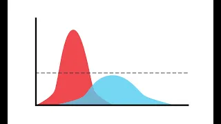
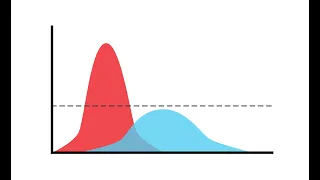
9 so which is probably the average speed of light somewhere in between and secondly, we can have a rough idea about how much spread there is about the centre which is typically summarised by a standard deviation. So to give you an idea of how the spread affects the shape of the histogram here are two hypothetical data sets where they have the same mean about 50. 50, 50 so this is about the centre of the two distributions but they have different standard deviations.
As is obvious the left one has a larger standard deviation right the spread around the centre is large whereas about the same location it's smaller right so this is the effect of different standard deviations on the histogram. Given the same mean if the distribution has larger standard deviation then the overall shape of the distribution looks kind of fatter compared to the distribution with the smaller standard deviation. Now back to the histogram.
We can also find out if the distribution is more or less symmetric about the centre or skewed to the left or to the right so in relation to this you can also find out about the presence of outliers which will have a chance to talk more about it but for this distribution it doesn't look like there is a serious violation in symmetry or obvious outliers and finally we can figure out whether or not there are multiple modes in the data by looking at the number of peaks which does not look like in this case either. So the mode of the distribution is easy to locate from a histogram. So to find the mode from a histogram you just need to find the highest point in the histogram.
Well it is not so simple as that mathematically speaking but visually that is where you find the mode and depending upon the number of peaks a distribution can be bimodal like in the graph on the left see you see that there are two obvious peaks in that distribution and if a distribution has more than two peaks as shown here right so it has three modes, looks like, and then we call this distribution multi-modal distribution. So here is the summary of things you look out for in a histogram. So when you look at a histogram you need to find the centre where the centre is and how much spread there is and you look out for if the symmetry is okay and at the same time you want to look at if there's an outlier or the outliers exist in the data set and also you want to take a look at if there are multiple peaks in a histogram.
So let's imagine that we have millions of data to plot a histogram and even though there's no right or wrong answers in terms of what the optimal number of bins or width of a bin should be as I said before but in general if you have large data set then it's better to divide the entire range into smaller bins. So for example here we have a histogram of data with 11 bins of some exam scores say that we have like thousands and millions of data set. So now let's increase the number of bins to 100 to see how it looks and we do this because we can and the data set is large.
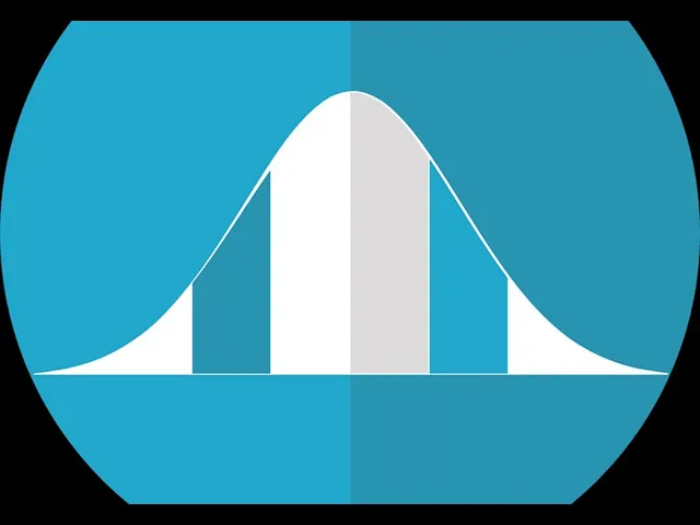
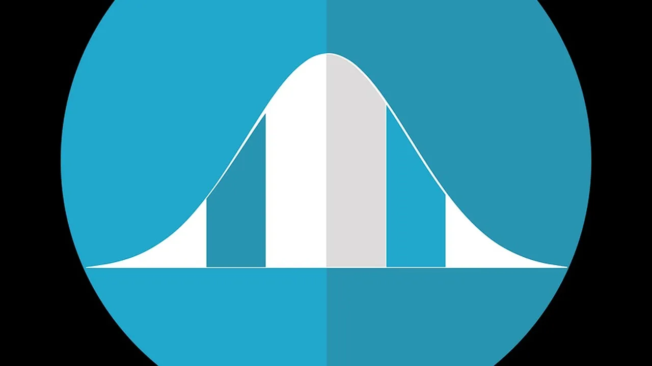
So now if we increase the number of pins naturally the width of a bin will decrease right and as the width of bin decreases then the histogram looks smoother see so if we keep dividing the range smaller and smaller then it will look smoother and smoother to the point where the outline of the histogram forms a smooth, continuous curve when the bin size approaches to zero and when the curve has the following features and we call the distribution a normal distribution. This is a typical shape of normal distribution. and by the way, you should not use the word "normal" in normal distribution like in an everyday sense.
so when a distribution is not normal then it is not an abnormal distribution. I sometimes see or hear people say the abnormal distribution to mean the opposite of the normal distribution. Well, it is not exactly the opposite anyway.
you should not use the word abnormal okay never ever say that in the context of statistics to refer a data set or distribution that is not normally distributed okay I said this. Now if a distribution is not normal then it is just a non-normal distribution or it is some other distribution with a different name all right? So when describing a normal distribution, data scores values go to the x axis and the probability occurrence frequency density sometimes they say this is a density go to the y-axis so as you can see from this curve normal distribution is denser in the centre and gradually thinning out to both tail ends from the centre hence the name bell curve.
and please note that those two tails never touch the x-axis and they stretch out to infinity in both directions. and from the mathematical point of view the normal distribution curve is describing how likely you will see a certain value in a data set. So for example, so if you have a data located on the x-axis here then the likelihood that you will see this data under this normal distribution is found on the normal distribution curve.
So the height of this data set to the normal curve determines the likelihood or the probability that you will see the data. So if you move to say like here the centre then the likelihood that you will see this data is actually this much okay and then this is basically the most likely observations you can see under this normal distribution. Because the normal distribution is symmetric around the centre and that is another feature of normal distribution so whatever score in the middle is the most likely observation you can have in a data set, assuming your data follow a normal distribution which will be the mean.
So what that means is that the more typical or mediocre values such as average are concentrated in the middle under a normal distribution. So these values are more likely to be observed in a data set. On the other hand, if you just go out to the tail then that's where you can find more extreme data right so they are kind of atypical data and the normal distribution so that is actually represented by the low likelihood, low probability of these data.
so these are extremes so if you think about like the exam scores right so say the usual exam score is 50 right so that is kind of at the centre then if you just go out too far away from the mean say you have like a 90 hundred and you have like a 10, 20. you do not find these scores quite often compared to the scores close to the mean right so that's actually what it means that the middle scores are more likely to happen whereas the extreme scores so the scores in the tails are more extreme and it is not likely that you see those data frequently. So another feature of normal distribution as I said briefly just before with all the central tendency measures the three central tendency measure we've learned mean medium mode have the same location which is exactly this in the centre of the normal distribution and the normal distribution is perfectly symmetric around these three central tendency measures under a normal distribution.
and another feature of normal distribution is that you can specify or characterise any normal distribution if their location parameter and well that is a scale parameter the spread parameter which is sigma so here this is actually a lower case of sigma. Remember the big sigma here? and that is the capital and then this is a lowercase of the sigma right and we use this um lowercase sigma to represent population standard deviation right so here this arrow represents spread the average spread in the normal distribution, which is typically represented by the sigma and then the mu this is another greek letter mu right representing the location parameter of normal distribution so that is just where the centre is right so that is the mu so that line is mu and that is sigma right so as long as these two quantities then you can specify the whole normal distribution curve mathematically.
In fact, there is no such thing as like a v with the normal distribution because depending upon this mu and sigma right there can be an infinite number of different normal distribution so here we have some a family of normal distributions showing and the mu is also called location parameter I said right because it dictates the horizontal location of the curve right so for example if we look at this blue one right so this blue curve here is specified so it has mu the mu of zero and the sigma square is 0. 2 right so sigma square is what? it is a standard deviation squared so this quantity is actually variance so sometimes the normal distribution is specified with the mu and the variance or standard deviation sometimes it is squared sometimes it is not but they just mean the same thing and see so the location of the blue curve is actually centred around zero.
That's where the mean of this normal distribution is but if we move or change the location parameter to the negative two then that becomes the green curve right green curve here and then you can see that the centre is actually moved by 2 to the left so now the new location is negative 2 for the green curve and if you look at the spread parameter, the sigma square is 0. 5 so it actually increased from 0. 2 to 0.
5 so it has the green curve has more spread and that is actually represented by larger. . .
the kind of a fatter graph right compared to the blue one right so the location parameter determines the location the horizontal location of the curve and the spread parameter determines the width of the curve and then we can also have the corresponding cumulative normal distributions curve and the cumulative curve has this kind of a characteristic shape looking like an s and these family of cumulative normal distributions here is actually the corresponding cumulative curve from this family of curve. So and again mu is the location parameter where it determines the location of cumulative normal distributions too see? You know the 50 of the blue is actually symmetric around the centre which is zero but if we move the centre by 2 to the left then the location parameter becomes negative 2 and the slope of the curve for the cumulative normal distribution also is determined by the spread parameter see the blue curve is steeper compared to the green one.
That's because the green one has more spread than the blue one. And another important feature of normal distribution is what's called the 68-95-99. 7 rule that relates the area or proportion under a normal distribution to the standard deviation.
So this rule applies to any normal distribution, so you might as well just remember this. So according to this rule the area under the curve bound by plus minus 1 standard deviation so here the mu again represents the mean of the distribution right the centre of the distribution and if you go out to one standard deviation so sigma here is a standard deviation. so mu minus one (standard deviation) is the score where this is the below.
. . so one standard division below the mean and the other score that is located one stand one standard deviation above the mean so when the normal distribution is bound by these two scores, then the area under the curve is 68.
And you can find 95 of the area under the curve within plus minus 2 standard deviations. So that is pretty much like the most data you will find I mean the most of the proportions under the the distributions say so within plus minus two so now you move another standard deviation far away from the centre and the area under the curve bound by these two scores now I just shade this okay so that is 95. And if you go out further to three standard deviations okay that's three standard deviations below the mean and three standard deviations above the mean then this area green area will be ninety-nine point seven percent.
So this is just a rule so you wanna just to remember it. So then what does this area under the curve mean and that is just the summed probability under the curve. So before I told you that and the normal distribution describes the probability that you will see a certain value.
So for example the exact probability that you will find this data under this curve is here right so that is just a single probability for this data set but when you say the area under the curve so that you want to calculate the area under the curve from this data to the negative infinity right so that means is that this is a summed probability that you will find this data or more extreme because the data to the left here right so that includes all the more extreme data from this data right so that's what that means so the area under the curve is a summed probability from a certain data point right and in this case because this is in more extreme side than this data set so you say the area under the curve in this red represents and the summed probability that you will find this data set this data set as big as this one or more extreme so that's what it means and by the same token this means the same thing so here if your data is located here then the exact probability just find this data under this normal distribution you can just find here right so that is a single probability but the area under the curve to this direction represents all sum of all the probabilities right all the other extreme values than this one so that is the area under the curve here. the summed probability that you will find this data or more extreme but that's what it means so if and what's the area under the curve in the middle again that's the summed probability that you will find between these two data sets so you add all the probabilities between these two scores so that's the meaning of area under the curve and this will become important later on when I try to explain the concept of p-values or alpha the level of significance Now that we have talked about the the proportions or the area under the curve, so let's just go over some problems and applying those the rules right so here we have a normal distribution so this big n represents a normal distribution and this normal distribution has the location for a mean of 50 and then a standard deviation of 10. So when you are given the specification of a normal distribution then what is the proportion of the blue region here given this normal distribution so that is the question.
So if you know the 68-95-99. 7 rules then this question is easy to answer. So this middle proportion so it's just bound by scores 40 and 60 here.
We know that the mean is 50 right the centre and then the standard deviation is 10 and these bounding scores happen to be one standard deviation so that's 50 minus 10 right and then this 60 is one standard deviation above the mean which is 50 plus 10 right so now we know that these two bounding scores are the plus minus one standard deviations from the mean and by the rule you know that the blue region is actually 68 percent. So here is another question for you. Now we have different normal distribution.
So now the mean is 75 and the standard deviation is 10. So in this case then what is the proportion of the shaded region with blue that is the question. So now we know that the 75 is the mean and you have to find out what are the two bounding values and it looks like a 55 is one 95 is another but this is a lower limit this is upper limit so we know that the standard deviation of this distribution is a 10 so the 65 is actually one standard division below the mean right so that is 75 minus 10 and 55 is another one standard deviation from 65 so that is actually 75 minus 20 right so that is a two standard deviation below the mean and 95 by the same token that is actually 75 plus 20.
right so this is a two standard deviation above the mean. So what that means is that these two scores are the scores that is plus -2 standard deviation from the mean so by the 68-95-99. 7 rule the proportion under this curve should be 95 percent.
Now we have a kind of a flipped problem where you're given the middle proportion so you are given the middle 68 percent and then you're given the specification of normal distribution here and the question is to find these two bounding values right contain middle 68 when the normal distribution has a mean of 40 and a standard deviation of 5. So this is kind of an inverse problem compared to the previous one right so now we know that this middle is 68 percent and by the 68-95-99. 7 rule we know that we can find the middle 68 percent within plus-minus one standard deviation from the mean right so we know that the centre is 40 so that is the given mean and the one standard deviation above the mean will be 40 plus 5 that's 45 right and the one standard deviation below the mean is 40 minus 5 so that's 35.
So the bounding values the lower limit and the upper limit is 35 and 45 for this question. Within 35 and 45 we know that we can find middle 68 for this distribution. So here is another similar question now the middle proportion given to you is 95 percent and you need to find out these two binding scores containing the middle 95 percent when this distribution has a mean of 20 and a standard deviation of 3.
again the mean is here 20. Now by the rule, we know that we can find middle ninety-five percent within plus-minus two standard deviations this time right because one standard deviation is three so that's three another three so plus three, plus three so this becomes 23 and then the two standard deviations from mean is 26 right by the same token you go two standard deviations below the mean of 20 that's 17 that becomes 14. right so the answer is 14 and 26 for this distribution.
The two values that you can find the 95 within. okay so here is another question but I'll leave it up to you to solve this problem and I'll put this question in this weekly quiz so the question is you need to find out the proportion of this distribution. So this distribution has a mean of 10 and standard deviation of 3.
and then what is the proportion of the distribution above 7 that is the question I so here again we have mean here right oh yeah means 10 and then where is 7? 7 is actually one standard deviation below the mean right so that is 3. see the single standard deviation here is a 3 and 7 is actually the score that is one standard deviation below the mean and the question is what is the proportion above seven so that is a question.
So have a think about it and see if you can come up with the right answer.