Given a data set, any raw observation or score can be transformed to what's known as z-score by subtracting the raw score from the mean of the data set and divide that difference by the standard deviation of the data set so this process of converting a raw score into a standard score or z-score is called standardising or sometimes it is called normalising but sometimes it can be confusing to use normalizing because it can mean something different too. Anyway this way any score can be expressed in terms of how far the score is away from the mean in the unit of standard deviation. So the raw scores above the mean will have a positive standard scores whereas those below the mean will have negative z-scores and so the mean itself then will have a z-score of zero so this z-cores are typically used for comparison purposes for example you may want to know you know where your body weight stands in the population so if you know the population mean and the standard deviation then you can convert your weight into z-score to see how different you are from the typical population weight, which is the population average weight and more generally so if a variable x follows a normal distribution with a mu and a standard deviation of sigma so here x represents any random variable and the squiggly sign is read "follows" so if a random variable x follows this big n represents the normal distribution and the normal distribution has mean of mu and the standard deviation of sigma.
So this whole thing on the left is read if a random variable x follows a normal distribution with the mean of mu and the standard deviation then it'll follow another normal distribution with the mean of zero and the unit standard deviation when every score in that random variable x is standardised by this z transformation or the the standardising process so we can convert any normal distribution into a single standard normal distribution so that's what that means. So here is an illustration of how a normal distribution becomes a standard normal distribution after a standardisation. So the distribution in light grey on the left is the original distribution following a normal distribution with the mean of negative two and the variance of 0.
5 so this is a variance instead of standard deviation because the reason that will become clear later on but so that x so that is the mu of the distribution and this is sigma squared okay not sigma. I told you already about before that sometimes and the normal distribution is specified by the standard deviation or the variance okay so the mean of the light grey distribution is here right and the standard deviation is about the spread is about here right that is actually square root of 0. 5 right standard deviation now if we follow the set transformation or the standardisation using the equation previously so the x is the all the scores of the original distribution in light grey right so you plug in all the numbers from the original normal distribution and subtract these scores from the mean of that distribution right which is negative 2.
and you divide this difference by sigma so because in this equation because of the square root that means this . 5 here is actually expressed in terms of variance instead of a standard deviation right so that's why I told you that this 0. 5 is variance instead of the standard deviation now if the x goes through this transformation then the resulting distribution is in this black distribution on the right which is the standard normal distribution so now all the scores are the z-scores converted to z-scores following the normal distribution of um with a mean of zero and a unit standard deviation so any normal distribution can be standardised to follow a normal distribution with a mean of zero and a unit standard deviation.
So let's work with some example question to illustrate how we can calculate z-scores in practice. So let's assume that we know the distribution of intraocular pressure in classical region and this is known to be a normal distribution with a mean of 17 millimeter mercury and a standard deviation of 5 millimeter mercury now you measured an intraocular pressure of a patient from the clinic and it turned out to be 27 millimetre mercury then what is the z-score for this patient's intraocular pressure is the question so this is a very simple question where you can just plug in the given numbers into that standardisation equation so the equation was z equals x minus mu and sigma so all you have to do is to plug in the numbers now what is the m the x so x is the original score that we want to convert into this z-score which is the patient's intraocular pressure 27 right and then you subtract this from the mean of the population which is 17 and you divide this difference by the standard deviation of the population which is five so now the top ten and that's two okay so the standard of the standard score of that you know the patient's intraocular pressure is two meaning that his or her intraocular pressure is actually two standard deviations above the mean which is considered quite high so the standard normal distribution has all the properties of normal distribution so you remember that the the 95 of the data would fall within plus minus 2 standard deviation under a normal distribution. So the exact value in fact is 1.
96 instead of a two. They just used the rounded number to make it simpler but the exact value is plus minus 1. 96 and so within these two values you can find the 95 percent of the data so these z-scores, as I said, tell you how far a score is from the mean in the unit of standard deviation so with that said, z score of 1.
96 or 2 um after rounding means that the score is actually two standard deviations above the mean whatever the original score is and the sign tells you if the score is below or above the mean and the total area under a z-distribution is one so when you normalise anything then it becomes one any normal distribution then the area under the curve is just a one and which is just basically hundred percent and the remaining area in both tail ends, see this kind of a reddish area is 2. 5 percent each because the middle 95 percent then then the remaining tail ends are five percent by combining these together so each because the normal distribution is symmetric around the centre so you split that five percent into exact halves to these two tail ends. So for various reasons and there has been a need to calculate any areas under the curve and this can be done using a calculus integration right if you want to do it by hand and by convention area under the curve in calculus is always um calculated from the negative infinity so from the far left here right up to a certain value z right so the area under the curve is starting from the left and to a certain score z.
So that's how you perform the integration in calculus and to make it easier to find the area under the curve instead of performing this calculus each time we need to find the specific area under the curve and people published a table of area under the curve like this one one for the standard normal distribution even about like 20 30 years ago I needed to use this table to find out a specific area under a standard normal distribution but thanks to the current computing power now we can calculate any areas under the curve by a few button clicks even with better precision. Anyhow the table provides the area under the curve up to any z-score of two decimal places ranging from negative 3. 49 to positive 3.
49 9. so this range I mean you can go further up beyond the 3. 49 but this table actually provides the area under the curve with a precision of four decimal places and it pretty much covers all the area under the curve right so it becomes just a pretty much one so they stopped at this range negative 3.
49 to positive 3. 49. So the table on the left shows the area under the curve of set distribution up to any negative scores and any negative z scores with two decimal places from negative 3.
49 up to the halfway, zero. On the other hand the table on the right shows the area under the curve of z distribution and up to any positive z-scores with two decimal places passing the halfway of zero to positive 3. 49.
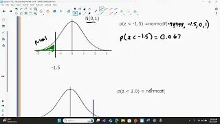
So using this table, then let's try to find the area under the curve at z score of negative 1. 96. So we're going to use the left table and to find out, you have to find out the z score of negative 1.
96. So the far left column are the is the list of the z-scores uh with a single decimal places so you find out negative 1. 9 first going down the column right so that is the negative 1.
9. Now you can find the remaining the second decimal places from the other columns so you're going down to find 0. 06 and the area under the curve is where these two you know the row and the column meets that's 0.
025 that's where the area under the curve at the z-score of negative 1. 96. So as we learned before right the left tail so this is basically the left tail and the area under the curve the left tail up to the z score of negative 1.
96 which was 0. 025 right so if we go back to this graph right so it is the at the left tail area up to the z score of negative 1. 96 and it was 0.
025 which is 2. 5 percent and from the table the number is exactly the same which is 0. 025.
So this is how you read the table to find the area under the curve up to a specific z-score with two decimal places. Because a normal distribution is such an important distribution, people came up with some technical terms to describe distributions breaking the properties of normal distribution. For example, we say a distribution is skewed to the left or right when the symmetry from the centre is broken and this typically happens when there are outliers in the data set.
Especially when the outliers are on the right of the distribution then this distribution has a positive skew or is said skewed to the right so as we just have seen and the distribution is pulled to the right because of the influence from the outliers right on the other hand when the outliers on the left of the distribution then this distribution has a negative skew or is said skewed to the left and as you can see and the distribution is pulled to the left when there are outliers on the left side of the distribution. Another term kurtosis is a term to describe the pointiness or tailedness of a distribution. So here is our normal distribution and when you have more scores close to the center then the resulting distribution looks fatter compared to the normal distribution we call this distribution platykurtic having a negative kurtosis where platy means "wide" or "broad" in Greek and a platykurtic distribution has thinner tails at both ends.
On the other hand, a distribution is called a leptokurtic looking more slender than the normal distribution and this distribution has positive kurtosis with thicker tails, meaning it has more extreme values at both ends than the normal distribution. So this illustration compares the part of box plot to the corresponding normal distribution side by side and as you can see the box plot is showing a perfect symmetry around the median for a perfectly normal distribution so um this first normal distribution is actually showing at the corresponding parts of the box so we have Q3 and Q1 which is the IQR right and by definition this IQR contains the 50 in the middle of the data as shown here and when the length of whisker is 1. 5 times IQR then the upper whisker is actually corresponding to 2.
698 sigma standard deviation and then the lower um whisker is actually corresponding to the negative 2. 698 standard deviation and up to that you know boundaries two boundaries each contains 24. 65 so if we combine these two together then it'll become 49.
3 right yes and 49. 3 percent plus 50 so that's 99. 3 and remaining tail ends will only contain 0.
7 so each will contain 0. 035 (I meant to say . 35 sorry) the 0.
7 percent so that's 0. 035 percent (again, . 35) so in decimal notation it'll be smaller.
And this one the bottom normal distribution shows the basically the 68-95-99. 7 rule where we can find 68 in the middle within plus minus one standard deviation and the remaining proportion will be then 32 percent right so each containing about 16 percent. So this is the kind of a side-by-side comparison between the box plot and the normal distribution.
So because normal distribution is perfectly symmetric around the centre the location of all three central tendency measures are the same under the normal distribution right? However when the symmetry is violated right so in box plot even even though this band is median if the distribution if a distribution is a normal distribution then it also represents the location of mean and the mode. But when the symmetry is violated in other words if a distribution is skewed then the locations of those three central tendency measures start to separate relative to the direction of skewness.
So here we have a normal distribution curve on top and the respective box plot representation at the bottom where Q1, Q2, and Q3 represent corresponding quartiles on each representation and as we have seen like before the box file is also perfectly symmetric around the median but when there is a negative skew right there the mean is most affected so the mean is pulled away from the centre to the left, then comes median in the middle, and the mode is on the right so when you have negative skew then you have this long tail to the left side which is represented by the long lower whisker of the box plot and also the location of the median is not central in the middle of the box and the upper whisker is shortened when there is a negative skew. On the other hand, the positive skew now will change the position of the mode and mean reversed with respect to the median so the location of the median is still in the middle of mode and the mean but then again mean is most affected it is really sensitive to the extreme values or outliers in the distribution. So with the positive skew the mean is pulled away to the right from the centre and it is actually shown by the elongated upper whisker in the box plot and then shortened lower whisker in the boxplot and again the location of the median in the box is off so the box plug can indicate the um the violation of symmetry from a distribution.