so in this 20 minutes I'm going to condense the better part of two chapters of theory that underlie the black Scholes Merton a very restrictive model in particular this idea that the model assumes that log returns are approximately normally distributed which is consistent with a model that the future stock prices are log normal returns are normal prices or log normal I'm going to show you exactly what that means and then finish by computing a confidence interval around the future stock price now the black Scholes myrn has many flavors or variations some of them quite sophisticated
but if we go back to the original black Scholes Merton model it is the elegant solution to a differential equation and that differential equation requires several assumptions I've listed all seven these are from John wholes chapter 15 which is my context here and you might agree with me that collectively these are very restrictive set of assumptions so this is in contrast to the binomial option pricing model that I've covered in previous videos in this playlist where that was a very intuitive process of building a tree a map if you like a potential future stock prices
that's an intuitive exercise and it's also flexible we were allowed to build in features like can the option be exercised early it's easy to build design those features into the binomial tree so the by Numa tree is not only intuitive but flexible well the black Scholes Merton is not intuitive really the most users it's more about black box pun intended but also it's not flexible a restrictive set of assumptions that when we break some of these we really don't necessarily get the right answer now I'm not going to go through all seven because some of
them will be familiar if you study capital markets theory things like this assumption here of no friction we do want to note that we're going to be in continuous-time as opposed to that binomial which were discrete steps so as part of the to calculus and the differential equation that's so elegant there is an assumption here of continuous time but I'm just going to highlight two because the first one is the topic or the rest of this video and I think this first assumption out of all seven is probably more important than all the others in
terms of practical importance but also if you're studying for a financial exam and you can see what it says it says that the stock price follows a log normal process with let's say expected return denoted mu as usual a mean or expected return is often omit denoted mu and constant Sigma well you know it's Sigma is that's standard deviation or volatility so this first assumption has two important parts well maybe three first is it's very important we know this is confusing and new learners we are talking about the price not the return it's the price
that follows a log normal process or follows a log normal distribution it's not the return and second notice we have constant or holes gone out of his way here to note that it's a constant volatility we don't practice volatility is not constant it jumps around is varying by time not all models require constant volatility for example GARCH however the black Scholes Merton does assume constant volatility so right away we're there we know that's probably unrealistic and then this assumption here is fairly draconian does the stock price really follow a lognormal process okay so that's the
first one the second one I'm sorry one two three the fourth assumption notice I put in brackets that's because although these the original set we can we can dispense with this one almost immediately right using a rule that serves us well throughout option pricing models and that is that the dividend generally subtracts from the stock price deducts its value I've covered the intuition about previously in the video I won't cope with that now we're gonna mean continuous-time so naturally we're gonna prefer a continuous dividend yield as usual denote it small Q and once we have
that it's generally going to be a subtraction in the black Scholes Merton and then we've handled it so we really don't need this and then so you could say we have six assumptions instead of seven if you like I think most of us view this set is essentially similar to the original set of black Scholes Merton would be safe to say the black Scholes Merton easily handles European options with a on a dividend paying stock okay so then this workbook can be downloaded as usual and then I'll just take a closer look but I won't
go too deep on the log normal but what Paul calls that log normal property of prices and in fact hit the previous chapter 14 the whole chapter is devoted to the Brownian motion or geometric Brownian motion GBM is a wiener process and the theory of the Wiener process so I'm just gonna give you real summary highlights here what we have here as part of this log normal property assumption that in essence assumes a geometric Brownian motion for the stock price the dynamics of the stock price there is an assumption about the dynamics of the stock
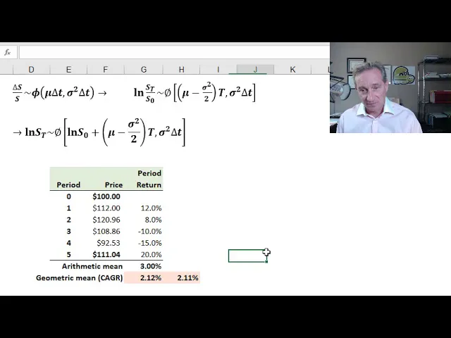
price in this model is that this return over a short period of time remember dealing with continuous space this return here Delta s over us you notice that that's a percentage but we're so where we we can look at this discretely but remember we're going to be in continuous time is approximately normal right that's the notation for normal distribution expect a return over short intervals with variance here for f prime candidates cfa candidates - this shouldn't be too surprising square root roll right it assumes and it assumes iid independent and identically distributed but if we
have that iid assumption that's the necessary assumption it's another assumption built in the model that volatility scales with the square root of time put another way variance scales linearly directly with time so we shouldn't be too surprised to see that variance just multiplies by the time interval here over short very short intervals now notice right here we have the natural log of the ratio here this is this could be called a wealth ratio today this could be today's stock price over yesterday stock price but here in the theory of the model it's actually very short
periods of time and hopefully this is familiar as the continuously compounded return right that's the return has that time additive properties very elegant to us we could also call it belt log return and so notice the important thing about this is it's not the price this is the return and the return is approximately normally distributed right so that's the key thing to keep in mind it's that the returns aka log returns are normally distributed therefore what that means is that the prices are log normally distributed returns normal prices log normal right so that we this
S sub 0 the initial stock price in the denominator here it comes out as a subtraction can go right into the inside the form the expression here for the normal variable and what we have then is the natural log of the stock price is approximately normal right so that's very important there that's not the stock price it's the natural log of this of the future stock price stock price at the horizon here could be one year or six months if that natural log that is approximately normal and so by definition of the log log properties
what that means is that the stock price itself as the price is logon or has a log normal distribution so the other part of this that is almost always confusing our new learners and is really based on the a theory upon which a whole chapter or more can be devoted is this expression in here the fact that the expected return here is not just the same mu here and a real short easy answer to that as whole puts it is to keep in mind that expected return has slightly different definitions so expected return the MU
itself is ambiguous and I prefer the other intuition here which is that volatility reduces returns so we have your an expression mu as the expected return and we subtract one half the variance and in fact in holes chapter I would call this an analogy he uses an analogy to explain this and I've used some of my own numbers here just to highlight how we can understand that analogy and I've done something very simple I take an initial price of a hundred over let's say five periods this could be five months if you like I just
made up some variation so that each period there is a simple return for each period right 100 goes up to 112 that's a 12% return over the period if we take the average of those period returns in my case I deliberately chose them so it's a nice round arithmetic mean of 3% by analogy we can think of that as the MU this mu here for the expected return on the other hand if I want to take the geometric mean which we can is the same as the compounded annual growth rate right I divide the one
the ending price of 100 11.04 by the 100 I raised that to the 1/5 power and subtract one and that's my geometric mean in other words my 100 compounded geometrically or the compound annual growth rate at two point one two percent gets me to the 111 point o4 probably seen this before this question of what's the average here of a series of returns is ambiguous until we get more specific but the point here in the analogy is that the geometric mean is always going to be less than the arithmetic mean the arithmetic mean is analogous
here to this mu and the geometric mean is analogous Tier two the arithmetic mean reduced by 1/2 the variance and in fact you'll notice I've done that calculation here I took the arithmetic mean and I subtracted the variance or the standard deviation of this series squared variance the new men are divided by two so I've performed that calculation here and just depending it's always going to come out as an approximation somewhere near my approximation here is going to approximate the geometric mean and the point is that let me put it as simply as possible volatility
erodes my geometric mean volatility of roads returns is how I like to think about it so over a short period of time the mean return is in fact mu times that very short interval but the expected continuously compounded return over the longer interval is actually mu minus reduced by one-half the variance so it is dragged down by volatility so that's the key expression here and then on the next page I only have two more in this video I just want to drive home this log normal property and remember what we've said is that the log
return right or the continuously compounded return is approximately normal all these shorthand notation there and what that mean is that the price the future stock price is a plot approximately log normal and here again in the worksheet and you can so this is dynamic including my bins I think they work here you can put in assumptions here I have an initial stock price of $20 mu of nine percent Sigma of volatility of 30 percent and then I one here time horizon and then what I've just done has been out here the future stock price right
not the return so the log return is approximately normal the future stock price here then will exhibit here a log normal distribution so you can see this prices these bins are based on the math here so they're not so clean but I've got looks like about eight dollars and twenty eight cents over here going up to forty three and then even more and so this is log normal hopefully you agree with me it's not symmetrical we can rule out normal distribution but importantly it's non-negative right so these are all positive values in the log normal
that mean the future stock price can't drop below zero so that intuition of a log normal price is starting to make sense and then also it has positive skew off the sheet here I calculated the skew because the skew of a log normal distribution is not hard to calculate and it's about point nine five above zero so we have positive skew the log normal will never be negative and also the mean is going to be greater than the median so another interesting fact about this future stock price so again when we go to talk about
what's the predicted future stock price under this model well we probably need to be more specific because maybe I'm just making this up maybe the median is somewhere close to the mode but we know the mean is going to be further off to the right so are we talking about the mean or are we talk about the median in this law log normal property of the stock price okay so final sheet final of four in this workbook and now I just replicate John Hall's example fifteen point one because if you really want to solidify your
understanding of this log normal property I would recommend going through this exercise and then he's also got like we do have some practice questions that apply it with other assumptions so this is a way to really understand all of this theory of the log normal property and what we have here is just the solution to the question what is a confidence interval around the future stock price and even before we go to do it knowing that the log normal property implies and here here I've gone ahead and have the plot under these assumptions of this
log normal it looks symmetrical but it's not knowing the log normal property we are not going to expect write a symmetrical confidence interval so I'm using John wills example 15 one initial price is $40 expect to return a 16% as usual assumptions are in per annum terms volatility or standard deviation 20% so I get this question a lot right we see the 20% we want to assume per annum unless otherwise specified this is not B there's no reason to expect this to be daily or monthly we should expect per annum and we do the conversion
and now we're going to construct the 95% confidence interval the confidence interval is a two sided interval so we want the two-tailed Devia and that's going to be 1.96 if you memorize some tip if you memorize some of the critical Z values you probably memorize 1.96 is the two-sided Z associated with 95% confidence and I have a function in there for that and then John Hall is the in this example it's projecting out a confidence interval six months in the future or half a year now I have here not part of the necessary solution but
here's my plot of the future stock price of that log-normal and the mean of that now I'm sorry the meeting of this is 42 I can't exactly place it 42 but then you'll notice the mean of this log-normal future of price distribution is slightly to the right of this slightly higher forty three point three but for the confidence interval right here I've just applied what's inside this normal variable for the log of the stock price right the log of the stock price has the normal property and so you can see natural log of the $40
plus my 16% minus minus one-half the 20% squared and it's just scaled by time so that gives me a not a number that's easy to intuitively understand because it's the natural log of the future stock price of three dollars and about seventy six cents my variance is very easy right per that square root rule volatility scales with the square root of time so variance scales with time simply multiplies the variance volatility squared by time to give me the variance of that normal variable and then the only thing I need to do is compute the confidence
interval so at the lower side I'm just now applying the very familiar pattern of confidence intervals right confidence intervals are expected value plus or minus Sigma the standard deviation which in practice is usually a standard error same thing standard error is a standard deviation multiplied scaled we scale the standard deviation by the Z value that's a function of our confidence and this case ninety-five percent or five percent right that's how we get confidence intervals that's the pattern that we used throughout and so you can see here that's all we do here take the mean of
that log of price add here 1.96 standard deviations standard deviation to the square root of this value that's our lower oh and I have just noticed that I've got these backwards from the label so I'm going to change out real quick I'm gonna make that the minus and make that the plus so I have lower and upper and so that's the but the that's the lower of the log variable so that to get back to my stock prices all I need to do is exponentiate these values here so just take erased to this value and
similarly for the upper and these match the solution in John Hall for his exercise 15 one we get then a lower bound on that confidence interval of 32 point 51 I think that's somewhere right about here and an upper bound on that confidence a told fifty six point six one I think that's some are right about there so that's the confidence interval for the future stock price ninety-five percent of the area under that curve and I also just noticed that even my label here is off by one so I'll these are swapped and that should
be g7 and g8 I think then I fixed it and so that's the confidence interval and if you can download the worksheet take a closer look at that but that is my attempt to cover the log normal property of the stock price and then the next video I'll show you the my black Scholes more option pricing calculator thank you if you like this video subscribe to the channel