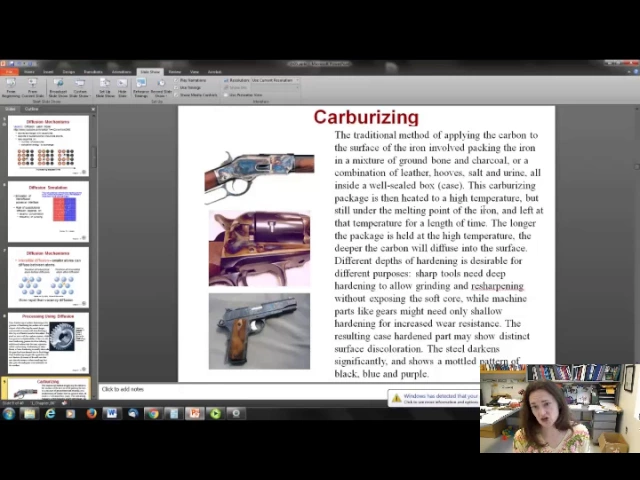
hi so um I'd like to talk to you about chapter five on diffusion we're not going to cover the whole chapter we we're not going to cover the non-steady state diffusion in any kind of depth but we will cover steady state diffusion and um temperature dependence of diffusion so first of all what is diffusion the um definition of diffusion is mass transport by atomic motion um so the atoms are moving moving around inside of material they're not still even in a solid material and they can hop from lattice sight to lattice site for a good video of that um I'd like to show you this one this is carbon atoms moving at the edge of a hole in graphine um and was taken in an electron microscope so here you go it's only about 15 seconds long and you can see the carbon atoms over here on the edge hopping around um and the motion of the atoms here on the edge of this little hole so that's really um kind of a fun thing to see there's tons of these sorts of movies out there on the web there's links in the PowerPoint presentation to three or four of them right there so if you'd like to watch more of those types of um images and movies taken in electron microscopes then that's nice um and they're there for you now of course no atom no atoms are still gas is is in liquid you might have heard of brownie in motion this is somewhat similar it's not as random walk because of course in a solid material they're hopping from lattice site to Lattis site so they're not free to go just anywhere um but it is kind of the same idea now in solids there's two ways that diffusion can occur you can either have a vacancy and the atoms can hop into the vacancy and we discussed how um there's always going to be a certain amount of vacancies in a solid material or you can have interstitial diffusion where you have a smaller atom moving through a material and it's hopping in the little vacancies in between the lattice sites um and so that's the two different mechanisms that diffusion can occur in so in inter diffusion let's say that you have some sort of material um on uh and the two different materials meet up at some Junction and then what happens is that if it's an alloy the atoms are going to migrate from regions of high concentration to regions of low concentration now similar to what you might have learned in thermodynamics or statistical mechanics this isn't for any profound reason okay it's just that things have a tendency to hop around and even if they hop around totally randomly what that's going to end up doing is melding them together so that it's uniform so this is very much the law of thermodynamics where systems tend toward disorder here on the left we have this very ordered system with one type of atom on one side and one typee of atom on the other and then after some time what happens is that the atoms have diffused around until they're mixed and that diffusion would continue if you followed it on towards the end of time until the two um solids were totally mixed and you couldn't tell where one started and the other finished so this is the concentration profile that you would see um after some time T if you watched them um migrate around now it's true that ALS so um atoms hop around within their own lattice sites as we saw in the movie in the semm movie that you're I'm sorry the electron microscopy movie that you just watched you saw carbon atoms hopping around within their own lattice um however from a macroscopic Viewpoint of material standpoint it doesn't matter too much when they do that I mean really why would you care most of the time if a an atom hops in the forest does anyone care um so self diffusion maybe not covered as much in Material Science just because it doesn't usually matter too much okay diffusion mechanisms um we watched the movie of how atoms are hopping around basically in vacancy diffusion what happens is the atoms are just moving to a vacant site um and and that's vacancy diffusion this happens when you have an alloy for example where the radi are similar and they follow the uh rules the Roth re Hume rules for substitutional solid solution that sort of thing that we covered in a previous lecture so this is for substitutional impurity atoms the rate at which they hop of course depends upon the number of vacancies if you have more vacancies you'll have more hopping and then there's also an activation energy for the atom to make that hop and um it'll depend on that as well this is a fun little simulation of inter diffusion across a um an interface and um you can see the vacancies and how they're hopping around and you can see that after a time um the the interface there starts to look more and more mixed and you get red atoms in the blue and blue atoms in the red regions um so the rate of the diffusion depends upon the concentration the frequency of jumping the activation energy and all those parameters now you can also have interstitial diffusion and that's when you have the smaller atoms diffusing um in a in a lattice of larger atoms um and they go in the little follows in the lattice sites so for example um a small atom like carbon moving through iron lattice um for example would go through interstitial diffusion and it would hop around from vacant site or hollow space to hollow space this has a tendency to be a lot more rapid than vacancy diffusion in other words two things don't have to happen to get this to happen you just have the intertial atom and it hops to another spot that was always vacant whereas in vacancy diffusion the the vacancy has to be there and then the atom has to hop um and the vacancy must move around so that's the difference um there's a little bit of addition there which makes the process um more rapid for interstitial diffusion now you might be wondering why we care about this at all and um the fact is that we've been using diffusion to alter the properties of materials for quite some time and we continue to do so um you might have heard of case hardening or Surface hard Harding and this is the process of hardening the surface of a metal object while allowing the metal underneath to remain soft and pliable so what that does is it makes a thin layer of harder metal at the surface this is really useful in steel okay if you have an iron with very low carbon content then um it's going to be much softer and then you can add carbon um and make it uh add more carbon to the mix and that causes the surface of it to be harder and more resistant to scratching and wearing this was originally known as carburising it's still known as carburising um but there's other forms of case hardening as well that don't involve carbon so the one involving carbon is called carbonizing so additional carbon is infused into the case um and then the part becomes a lot more resistant to fracture um and uh strains on the surface so if you're into any kind of antiques on some antique guns you might see this sort of mly bluish purple finish um and then you know that that part has undergone carburising the traditional method to do this um involves packing the iron in a mixture of ground bone and charcoal or um some somewhat grosser combinations of leather Hooves salt and urine all of which of course contain carbon and then putting it in a well sealed box or a case which is why it's called case hardening um and then the carbonizing package is heated to a high temperature but still less than the melting point of the iron and then left there for a long period of time and then of course the longer that you hold it at the high temperature the deeper the carbon goes into the surface um different depths of hardening might be desirable for different purposes if you need a sharp tool you might need deep hardening um so that you can grind it and resharpen it without exposing the soft core um but things like gears or gun parts might only need a shallow hardening for wear resistance um processes that use diffusion now are doping of semiconductors so for example if you want to dope silicon with phosphorus for an N type semiconductor then you could deposit phosphorus layers on the surface and then heat it and then this phosphorus will diffuse into the semiconductor and make it um an end type semiconductor actually change the electrical properties so um diffusion still gets used a a lot okay so how do we model diffusion first of all let's quantify the quantity known as flux okay your textbook uses a j to indicate flux for whatever reason the flux is going to be the moles or mass that diffuse through some cross-sectional area within a certain unit of time and the SI units of that are either going to be moles numbers or kilograms um per area per time sometimes they use centimeter squared for the area and sometimes they use meter squared um but it will be some SI unit of area per unit time this is measured empirically um basically you can make a thin film or a membrane of some known surface area and then impose some sort of concentration gradient on it so that you put more of whatever you're trying to diffuse on one side and the other and then measure how fast this happens um moves across the membrane in that unit time okay let's cover steady state diffusion steady state diffusion is when the diffusion is independent of time okay so you're having diffusion across for example some thin membrane and on the left hand side we show a concentration one and then on the rightand hand side we show some concentration too in steady state diffusion will mean that the concentration profile across that membrane will be linear okay so you have some thickness Delta x to the membrane that it's diffusing across and then you have a linear concentration profile across the membrane this is covered by fix first law of diffusion fixed first law of diffusion says that J is equal to minus D times the derivative of the concentration profile with respect to the spatial coordinate okay so here D is the diffusion coefficient the units of it our area per time me squar per second for SI units and then DC DX that derivative can also be approximated for steady state diffusion cases as the Delta C the change in the concentration over the um the membrane divided by the thickness of the membrane here given as X2 minus X1 okay when is this valid okay well not much I'll tell you that but um it's valid if you have a constant supply of your dopent um for example if you have some constant pressure of gas that you're flowing through um and constantly keeping the gas at that level then that would Supply you with a constant amount of dopen over time and that would be satisfied or like in the example that I just showed if you have a really thin membrane that's separating two dissim dissimilar but basically infinite environments so if you just have tons of your dopen available um and this sort of infinite Reservoir which is very reminiscent of statistical mechanics by the way then that um satisfies it also if you look at really short time scales what could look um of course things look linear when you only look over short time scales so if you only look over time short time scales even something that's nonlinear can look linear for a brief period of time all right let's work on an example problem um for uh this steady state diffusion the example here um is taken from your text and it's a phosphorous stoping of silicon like for a semiconductor um as we mentioned earlier okay so one way to manufacture transistors is to diffuse impurity atoms into a semiconductor material such as silicon let's suppose that we have a silicon wafer and it's 0. 1 CM thick the wafer originally contains one phosphorus atom for every 10 million silicon atoms and it's treated so that there's 400 phosphorus atoms for every 10 million silicon atoms at the surface so calculate the concentration gradient in atomic percent per centimeter and in um atoms per centimeters cubed per centimeter given that the lattice parameter of silicon um that's the lattice bacing is 0. 437 okay so what is this problem asking us basically it's asking us to calculate that D CDX or the Delta C Delta X for two situations that basically they want two sets of units on that concentration gradient and the first set of units will be in terms of a percent and the second will be in terms of number of atoms so let's do this so here's our Delta C Delta X and what we want is we want to calculate the concentration gradient over the slab of silicon from the top to the bottom okay we're going to assume that the bottom is um going to maintain that constant value that it originally had the one phosphorus atom for every 10 million silicon atoms okay we're going to assume that it it stays at that value whereas the top that's where it's getting dosed with the phosphorus and that's where the concentration is going to go up to 400 phosphorus atoms for every 10 million silicon atoms so the way that we're going to calculate that is we're going to it first ask for the units in terms of a percentage so we'll calculate the fraction and then multiply that times 100% to get the concentrations um and then we'll divide that by the thickness okay so here we go C for the bottom is going to be 100% times one phosphorus atom over 10 million silicon atoms and that gives you 1 * 10us 5% and then for the top you're going to have 400 phosphorus atoms divided by 10 million silicon atoms times 100% And that gives you 4 * 10 minus 3% so your concentration gradient in terms of units of percent Delta C over Delta X will be the difference in those two percentages divided by the thickness and that gives youus 0.
399 per per centimeter for your concentration gradient okay now I've set this up so that my concentration gradient is negative and that's because of the way that fix first law is structured remember the equation said that J is equal to minus D * D CDX and so um we'll set it up so that that multiplies out to become positive for J now we need to switch the units so that we're dealing with a mass um it asks for the um atomic um and then the oh I'm giving everything I'm giving the number percent and then I'm giving the mass um concentration gradient as well so I'm just giving you everything okay so how do we do this how do we switch these units over so it gave me the lattice spacing of silicon basically that's our a value that's how big one side of that cubic um unit cell is so silicon forms a diamond cubic cell um and it's got eight atoms per cell so the volume of a single cell would be that 0. 54 nanometers and then cubed now I'm going to have all my units be in centimeters so I write that as 0 54307 * 10- 7 cmers and then I Cube it and when I do that I get 1. 6 * 10- 22 cm cubed for one single cell now the total volume that I have is going to be um how much volume is occupied by that entire thing so if I have 10 million atoms and I know that there's eight atoms per cell then I can use that to figure out the number of cells and then I can multiply the number of cells times the volume of one cell and get my total volume so here I have 10 million divided 8 * 1.
6 * 10us 22 um centimet cubed per cell and that gives me 2 * 10- 16 cm cubed for my total volume so now my concentration at the top is going to be 400 phosphorus atoms divided by my volume okay okay which gives me 2 * 10 18th phosphorus atoms per cenm cubed and then for the bottom I've got one phosphorus atom divided by that volume and I get 0. 005 * 10 the 18th phosphorus atoms per centimeters cubed so that's a a number concentration per volume and then I want to calculate my Delta C Delta X so I subtract those two concentrations 05 minus 2 um and then divide that by my thickness . 1 um and I end up with 1.
n95 * 10 19th phosphor phosphorus atoms per centimet cubed per centimeter which is the units that it asked it for in the problem if there's other problems that ask you to convert that to a mass then you just use the atomic weight the atomic weight of phosphorus is 3. 97 grams per mole and I can use that to convert from a number of atoms um to a mass which I've done here um I'll leave that as an exercise for you to convert from atoms to grams it's uh tough but it it's it's not very tough but if you have questions I'm happy to answer them okay another example problem for you that does the full thing there we were just calculating the concentration gradient I'd like to also show you how to um do the full fix fixed first law problems so this example problem I also took from your book a thick welded pipe 3 centimeters in diameter contains a gas um including 0. 5 * 10 20 nitrogen atoms per cubic cimer on one side of a 0.
001 CM thick iron membrane the gas is continuously introduced to a 5 cm length of pipe the gas on the other side of the membrane contains 1 * 10 18th nitrogen atoms per cubic centimeter calculate the total number of nitrogen atoms passing through the iron membrane at 700 celsius if the diffusion coefficient for nitrogen is 4 * 10- 7 cim squ per second okay so um let's think about all this and put this together the first thing that I can do is I can go ahead and calculate my concentration gradient Delta C Delta X okay so in the problem it gave me the concentration of the nitrogen gas on either side of the pipe um and so I'll plug that in here to my Delta C so I have 1 - 50 * 10 18th atoms per centimet cubed for my nitrogen concentration um on either side of 0. 001 centimeter um pipe okay so when I calculate that Delta C Delta X I get minus 49 * 10 21 atoms per centimeter cubed per centimeter so that's my concentration um gradient now my full equation for fixed first law is J is equal to minus D Delta C over Delta X so I've already calculated Delta C over Delta X and I put that into the equation and then the problem told me that the diffusion coefficient for nitrogen um that's D is 4 * 10 - 7 cm s/ second so now I put that in and then that gives me my value of J which is 1. 96 * 10 16 atoms per centimeter squared per second okay but now the problem asks the total number of nitrogen atoms passing through the iron membrane at 700 C okay so that's the total number passing through so J remember our definition of j was one over the area times the amount of mass moving through in a unit time DT so if I want just the mass moving through in a unit time then I have to multiply J times my area to get that value so here J time a would give me my dmdt now the area that it moves through remember this is a pipe a cylindrical pipe and it's moving through that outer curved surface of the pipe so we need that area you can imagine the nitrogen diffusing from the inside of the pipe to the outside of the pipe moving out radially so we need the area of that outer curv surface and the formula for that is pi * the diameter time the length and that would give you the area of the outer surface of the cylinder so that gives us Pi * 3 cm * 5 cm which is 47.
1 square cm so then I plug that in for my area and multiply it times J and I get 9. 24 * 10 17th atoms per second which is the answer to our problem remember you always pause the video and ask me later if you get confused okay so of course um we talked in another lecture about how the number of vacancies in a material goes up exponentially with temperature and we also talked about the link between diffusion and the number of vacancies so since um the number of vacancy increases with temperature it makes sense that there would be a temperature dependence to diffusion the equation that relates um the diffusion to the temperature relates to that diffusion coefficient D and D that you would plug into fixed first law you can figure out um the temperature dependence of that coefficient using this equation D time e minus QD over RT or QD over KT if your units are different so if the the activation energy can be given that's QD um and that's how much energy it takes to create that vacancy to get the diffusion to happen and that's equal to Jews per mole and sometimes it's given in kilog per mole or it can be given in electron volts per atom um if you give the units in electron volts per atom then instead of RT where R is the gas constant you plug in KT where K is a bolts sp's constant um the temperature is in kelvin and D is just a little pre-exponential that's usually derived um from experiment or figured out from experiment okay so here you can see from this graph the exponential dependence on the temperature that the diffusion coefficient has um here along the Top Line you can see the temperature has been plotted um the logarithm of the temperature has been plotted and then here on the bottom it's one over the temperature that's been plotted um so you can see that this on this graph it forms these straight lines um so you can see here a couple of things to knowe the diffusion for interstitial diffusion is greater that diffusion coefficient is greater than for substitutional um diffusion so here it's comparing carbon moving through iron in a couple of its different um forms to aluminum and aluminum or iron through iron or iron through iron okay so basically um self diffusion so if you look at that then you can see that the values here for D range from 10us 20 here on the bottom of the scale to 10- 8 on the top and you can see that the um the values for the diffusion coefficient are a lot lower for that interstitial diffusion of carbon and iron than they are for the substitutional diffusion of the metals um normally less energy is required to squeeze an interstitial atom past the surrounding atoms so of course the activation energies are lower for interstitial than for vacancy diffusion there's a chart in your book um a table in your book table 5. 2 that lists um the values of D that she would plug into that equation d e minus QD over RT um and also the activation energies that have been determined experimentally for um these various um sets pairs of of diffusion so here's the diffusion species on the left that's what's diffusing in the second column it gives the host metal so here you have carbon that's what's diffusing through the iron that's how you read the chart you can see that um for the values of carbon and iron the values that you read off over here 10us 10 10- 11 10- 12 and you can see that goes all the way down toh 10us 22 for copper and nickel so you can see there's a huge range of values for um these diffusion coefficients all right let me do an example problem for you on the um temperature dependence of diffusion so here suppose that interstitial atoms are found to move from one site to another at rates of 5 * 10 8th jump per second at 500 C and 8 * 10 the 10th jumps per second at 800 C so calculate the activation energy um for the process okay so here we're going to use our equation D is equal to d e minus QV over KT um and then what we're going to do is take the natural log of both sides of that equation um so we have Len of D is equal to Len of D minus QD over KT okay so that's the equation we're going to be working with what it gives us here are two different temperature and diffusion coefficient pairs but it doesn't tell us what the material is so we don't know if it's carbon and iron or what we have no idea um so what we have is basically two equations and two unknowns so since we have two equations and two unknowns we can solve so let me show you how that goes here we have um Len of D1 equals Len of D minus QD over kt1 and then we have the same equation for the second pair we're going to subtract those two equations to get rid of our unknown so our unknown here is the D we definitely don't know D but that gets subtracted out when I subtract my two equations so then I have Len of D1 minus Len of D2 equals minus QD over K time um 1/ T2 1 over T1 minus 1 over T2 so that's that's what we're doing there now I just plug in the values given to me in the problem the 8 * 10 10th 5 * 10 8th and the two temperatures which I have to switch over to Kelvin 773 and 1073 Kelvin and then I solve for QD and when I do that um as long as I use boltzman's constant here I'm going to get my units of QD in uh EV so I've got the EV per Kelvin units of boltzman's constant 8.
62 * 10us 5 EV per Kelvin for boltzman's constant and that gives me my activation energy in EV 1.