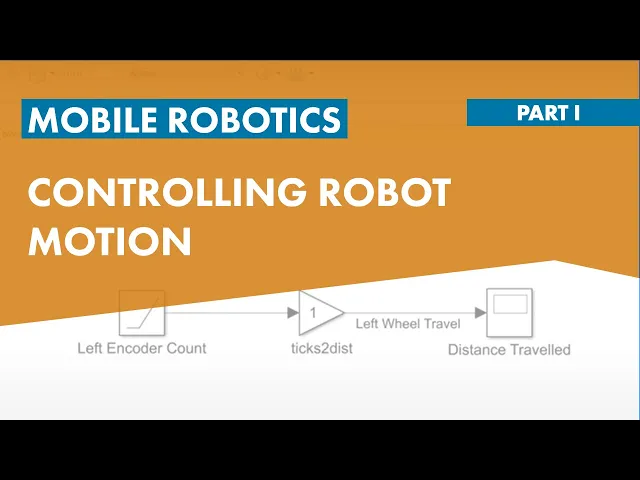
in this video we are going to learn how to control robot motion that is to move it forward or backwards consider a differential drive robot as shown here a differential drive robot is one that is actuated by two motors a left and a right motor our first aim will be to move this robot for a prescribed distance for example here we have a robot that moves in horizontal direction for a prescribed distance of 1 meter these kinds of processes where we use the distance traveled by the robot to determine its position is called dead reckoning in general this falls under the problem of knowing where the robot is and this is called localization one possible way to do this is to use what are called encoder sensors to compute the number of rotations of the wheel to determine the distance traveled other popular ways to achieve localization are to use other sensors such as GPS in I am you a camera lidar etc in our example we will stick to using the encoder sensors to implement the dead reckoning algorithm with the final goal being to move the robot in a straight line for 1 meter we will use simulate to do this but first what is similar let's look at this from a high level many engineering applications such as space communications automotive energy and robotics usually involve tasks that require you to write a lot of code to solve a problem in Simulink we express this problem as a block diagram using what are called models models represent various components in our system in our case we want to model the system of equations for a differential driver robot and the logic to move it here are the input sensors the calculations the robot logic and a way to visualize the simulation once we have built the model we run our simulation checking results we see the robot position and the fact that it moves for 1 meter we also see time traces of various variables plotted versus time such as distance traveled and velocity this is because in simile all our simulations are time dependent using simulations like this you can explore what-if scenarios there are impractical to perform in real life but simulation can only take you so far at some point you need to be able to perform these tests with real hardware this is also possible in simile using hardware support packages we will talk about hardware support packages later on in this video okay now that we know at a high level what similan is let's go back to our original problem of moving the robot for a prescribed distance to understand how to do this we will talk about the basics of encoder sensors understanding how to calculate distance using encoder sensors implementing a dead reckoning algorithm given a prescribed distance to travel how to move the robot by that much distance we will then test our dead reckoning algorithm using simulation and finally we will look at verifying the algorithm on an example Hardware first let's talk about the encoder sense of basics assume that we have a wheel like this an encoder is a device that is connected to the wheel motor shaft now if we rotate this wheel by one full revolution which is 360 degrees the encoder counts discrete number of ticks corresponding to the rotation in our case nine ticks by the encoder means one full rotation or 360 degrees we can use this information to determine the number of wheel rotations we count the total number of encoder ticks and divide that by the tick count per rotation value in our example this is nine in reality this could be found on the manufacturer datasheet of the encoder now we know how to compute the number of wheel rotations with an encoder but how is this useful to calculate distance a device that is used to measure the distance traveled is also called an odometer let's see how to use encoders to build an odometer let's take our wheel again this time when we rotate this wheel one full rotation which is 360 degrees the wheel center would have travelled a distance equal to the circumference of the wheel this circumference is given by the formula two times pi times R where R is the radius of the wheel knowing this we can say that the total distance traveled by the robot equals the number of rotations times the circumference we can then substitute the number of wheel rotations by the equation in the previous slide where we compute wheel rotations using encoder ticks it is important note that the tick count per rotation and circumference are fixed values for most robots and need to be determined only once this is because the tick count per rotation for any given encoder sensor is constant as noted in the manufacturer datasheet the circumference depends on the radius of the robot wheel this is also going to remain constant the only variable is the total number of encoder ticks we can think of this quantity as the input to our system the output of the system is the distance traveled let's see how we can implement an odometer in simulator the input to this system are the encoder ticks and the output is the distance traveled let's switch to MATLAB to get started with similar select the Similan icon in the home tab of the MATLAB toast room this will open the Simulink start page the Similan start page contains a set of model templates which are useful for different applications it also provides access to product examples recently open files and templates the diva of previously created clicking a template will create a new Simulink model based on that template the Similan model window is where you visualize and simulate a block diagram of your system to create a new model select the blank model template over here to add blocks to this blank model let's open the Simulink library browser by selecting the library browser icon on the tool strip the sibling library browser displays libraries in a list on the left hand side to see the blocks container library select the library name the blocks inside the library are listed in the right column to add a copy of the library block to a model drag the block from the library browser to the block diagram in order to build our first model let's copy the following blocks let's go into the sources library and choose the ramp block click and drag this into the model we will use this block to simulate an encoder sensor a ramp means the signal rises with constant slope this is representative of an encoder behavior when the robot is moving in a straight line the next block that we need to add is the gain block so let's go back to the library browser and under the math operations library let's choose the gain block drag and drop this in the model this skåne block is used to convert the encoder ticks into distance traveled since the output distance travelled is a constant multiplication factor of the input in quadratics value we use a gain block and finally we need to visualize the output of the system so let's choose a scope block from the sinks library it's going back to the library browser and under the sinks library let's choose a scope block and add it to our model now we just have these blocks how are they going to interact with each other we need to connect them the output of the RAM block should be the input to the gain block to connect these two blocks left-click on the put port and drag it to its destination and let's do the same for the gain block and connect it to the scope next it's usually a good idea to rename block in signal names to enhance the readability of the model to rename the block click the block label and edit it let's rename the ramp to left encoder count this signifies that it represents the left wheel ticks let's rename the gain block to ticks to distance and the scope block a distance traveled it's also rename the signal that is the output of the gain block the left wheel travel to name a signal click on the signal and type in the name recall that we have just dragged and dropped these blocks connect to them and label them next we need to define their parameters to make them describe our system or equations we will leave the RAM to be at its default values for the gain block we will specify the equation that we delivered in the presentation so let's double click on the gain block to open the block parameter dialog and let's specify the parameter values as 2 times pi times wheel are divided by ticks per rotation note that the wheel R and ticks per rotation are variables and need to be assigned to do this let's click on the ellipses besides the dialog and choose the create variable option and let's select ticks per rotation set the expression to the value in our case let's set this to an example value of 360 so like I am doing here this means that is 360 takes for one rotation lets it create and let's say ok let's repeat the process for wheel r and set this value to be point zero five to now let's hit apply and let's switch back to the MATLAB window for a second to see that these variables have been created in the command prompt as you can see ticks per rotation has been set to 360 and wheel R has been sent to 0. 005 - let's go back to similar curve we can resize the gain block to see the equation created here just like I am doing right now let's also visualize the input signal so let's create a copy of the scope block to create a copy right click on the block and drag it let's rename this block to be encoded ticks and now let's connect this to the output of the ramp block to connect a signal right click on the signal and drag now let's run our model in run your model by clicking on the green Run button on the tool strip let's open the encoder tick scope block we see that the encoder has 10 ticks now let's go and open the distance travel scope the distance traveled is close to 10 raised to negative 2 meters the way the ramp block is set up in outputs one tick per second so let's run this simulation for 360 seconds let's go back into the model and let's and change the simulation time up here now since our ramp block outputs one take per second if we run our simulation for 360 seconds we expect our encoder to reach 360 ticks which is equal to one wheel rotation so let's run this model again and now let's view the encoder stick scope we now see that the encoder takes his reach 360 let's go back to the distance travel scope we see that the distance traveled is about 0. 3 to 5 meters let's compute our circumference in the MATLAB command prompt let's switch back to MATLAB we know there are circumference is equal to 2 times pi times the wheel radius which is 0.
05 to we see that these results match let's look at the big picture we can now use this simulation to calculate the distance traveled for a given number of ticks or back calculate the number of ticks required remove a distance the next question would be this is for the left wheel alone what about the right wheel what about the robot as a whole let's go back to the presentation and look at this here is an example robot we are looking at the top view of the robot so the red block is a robot body and the black blocks are the wheels suppose the start and end points are here now when your robot moves from the start to end like this the distance traveled by the right wheels and the left wheels are different as shown here however we are interested in the distance traveled by the centre of the robot which is denoted by the green line this is easily obtained by taking the average of the left and right distance traveled we have already implemented the distance traveled equation for the left wheel let's reuse this for the right wheel and complete the calculation by taking the average let's go back to our model let's copy the left wheel blocks you can copy a group of blocks by selecting the group of blocks that need to be copied right clicking and dragging just like we did earlier now let's rename these blocks to be the right wheel blocks so the ramp block would be the right encoder count the output signal of the gain block would be the right wheel travel and the scope would be right in correct tricks now we need to take an average in order to take the average we need to first add the two quantities and then divide them by two so let's go back to the Similan library browser and from the math operations library let's choose the add block and drag it in to our model now let's connect the left wheel travel and the right wheel travel to the add block delete off this portion of the signal for a quick second dear now after adding the two quantities we need to divide it by two dividing something by two is the same as multiplying it by 0. 5 so let's add a gain block from the Simulink library browser and set the gain parameter to be 0. 5 another easy way to set the gain parameter is by entering it into the banner that cap pops up when you insert the block into the model now let's connect the add block to the gain block and the output of the gain block to the distance traveled scope now let's test for the scenario where the robot is rotating in one place that is the left wheel is rotating in the forward direction and the right wheel is rotating in reverse at the same speed so let's set the ramp input slope for the right wheel to be negative one let's open up the right encoder count ramp block and set the slope to be negative one now let's run the model let's open up all the scopes we see that the left and right encoder scopes are non zero values that means the wheels are rotating however the distance traveled is zero because the robot has technically not moved anywhere else it has just been rotating in one place we can use this model to do tests from actual sensor data to figure out how far the robot has moved so given the left and right encoder values we have successfully computed the distance traveled let's go back to the presentation for a recap we just built our first sibling model we use the graphical modeling environment to build an odometer from encoder sensor inputs we see that similan can be used to generate example inputs and look at outputs in addition to this it can also be used to implement mathematical equations the simulation environment helps in testing what-if scenarios for example using a model we can check how far the robot has moved given an encoder input the next step is to implement the actual algorithm so far we have been implementing math what about logic many of the robotics algorithms involve logic and more based operations let's take a simple example based on the model we just built what if we want to monitor the distance traveled and then stop the robot once we have reached one meter if we visualize this in a flow chart first we begin execution of the algorithm then we will have the robot move forward next we check if the distance traveled is greater than or equal to one meter if it is we have already reached our goal and we should stop if not we move our robot forward again we can move the robot in a desired fashion by controlling two variables V which is the linear velocity of the robot representing how fast the robot is moving in a straight line an Omega which is the angular velocity and that represents how fast the robot is rotating in one place so to move the robot in a straight line we set V equal to a nonzero value and stop we set it to zero Omega remains zero for straight line movements since we are not rotating the robot let's go back to similan and see how we can implement the flowchart logic to move the robot for one meter in the model that we are working on we will use state flowcharts to build logical part of our algorithm state flow is great at modeling modes of operations and making logical decisions to add a new chart to a model let's open the Simulink library browser and scroll down to the state flow library and from the stateful library let's drag the chart option into the model this chart should take in the computed distance traveled as input and then output a velocity value let's double-click on the chart block to open up the state flow chart recall that we have two modes of operation in our algorithm a move forward mode and a stop mode model this we will use States to add a state to the chart select the state option on the toolbar on the left and drag it into the model the first state of the chart is the default State this is denoted by the default transition here which is where the program execution begins we can add a comment here by double-clicking on the transition and editing the question mark to add a comment add the percent sign and then type out your comment let's call this the start to add the second state let's make a copy of the first step copies of states can be made in the same way like we make copies of blocks in Similac now we have two states we must label each state with a valid name valid names are any alphanumeric or underscore characters without spaces and don't start with the number look at the link in the resources section to get a full list of rules for naming a state let's name the first state as the move forward state and the second is a stop step now we need to define the state execution statements what should these states be doing they need to be controlling the velocity V move forward should set the V to 0.
1 and stop should set the V to zero so let's type in V equals two point one in the move forward state now we see the state flow automatically adds another word namely entry to the description this means that state flow will execute the statement once when it enters the state we can see this better when we run the model for now let's also set the velocity in the stop state to zero so V equals zero and as you can see the entry word has been added here as well next we need to define the condition at which we will transition from the move forward state to the stop state we already know this condition to be that the distance travel has to be greater than or equal to one meter for this to happen we know that our robot has to stop once it reaches the 1 meter mark and hence the transition condition will be that the distance traveled is greater than or equal to 1 meter to define this we will use transitions to create a transition move your pointer at the edge of the move forward state until the crosshairs appear and then click and drag until the destination which in our case is the edge of the stop state and then release the mouse button we have now defined a transition path next we need to define on what condition does this transition happen so let's double click on the transition to see a question mark pop up let's type in the condition that we discussed earlier which in our case would be dist travel this is greater than or equal to 1 then click outside to see that state flow automatically adds square brackets around the condition this is the necessary syntax most times state flow does this first automatically other times do note that the conditions need to be enclosed in square brackets now our algorithm is complete next let's think what where the district um and where the V value is going to these are input and output variables in our chart and they need to be defined as such to do this let's go to the View tab on the tool strip and select the symbols option this pulls up a pane on the right hand side of the screen that has the symbols already over there here we can see that stateflow already recognizes these as unresolved symbols we can resolve these by clicking on the exclamation button on the top over here just like I am doing right now then we can verify if stateflow has resolved them correctly and as we can see this travel is an input and V is an output which means the state froze right let's go back up one level in the model through the breadcrumb over here now when I resize a chart you can see that an input in an output port has been created to the state flowchart and now looks like any other similan block which accepts inputs and outputs where does the district value come from though we have already calculated this here as the input to the distance travel scope so let's add the chart to our model again recall you can connect a signal by right-clicking on the signal and dragging it now let's connect the output of the Chart V to another scope so let's make a copy of the distance travel scope and connect the output V to it and let's rename this as velocity now let's remember to change the slope on the right in code account ramp block to positive one to signify that our robot is moving in a straight line let's change the slope to 1 and hit enter now let's run the model and let's take a look at the distance travel scope as you can see this the value on our distance travel scope is a lot less than 1 recall that our algorithm is only doing something interesting when the distance traveled becomes greater than 1 so let's run the model for a longer time so we can see what happens so let's go back and chain the simulation time on the top tool strip to 2000 and now let's run the model again now we can see that the distance travel has gone beyond 1 let's approximately make a note of when it crosses 1 which looks to be around 1100 let's open the velocity scope here we see that initially the velocity is 0. 1 and then at around 1100 it jumps to zero so our algorithm works let's go back inside the state flow chart and understand this a little more let's right click on the disk travel transition and set a breakpoint when the transition is valid just like I am doing on the screen right now and now let's run the model again we see that the execution has stopped in the model and it is soft around eleven hundred and twenty so we were correct that this condition was true around eleven hundred now we can use the step mechanism here to see a step by step execution of our algorithm so let's step through this once we can see that it has now moved to the stop sale we can create breakpoints this way in various parts of our chart to help us debug our algorithm let's hit the Run button again to finish the execution we have now successfully created a dead reckoning algorithm let's go back to the presentation and do a small recap we just built our first state flowchart we use States to describe the two modes of operation of our robot and we use transitions to test for logical decisions in our algorithm in our example the moment our robot crosses the 1 meter mark the velocity value went to zero however we can note here that our input sensor is just a simulated value this is an open-loop system which means that there is no connection established between our robot velocity and the input encoder value we will be able to test for more scenarios if we have the input encoder value to reflect a real system output in other words the distance value should stop increasing as soon as the robot velocity reaches zero to do this we will be using the mobile robotics training library that is provided with this training this library like any other similar library has several blocks in it it has a robot simulator that can help us visualize a robot given right or left wheel angular velocities note that these are real angular velocities which are different from the V and Omega values we discussed earlier we also have a few utility blocks for example to convert V and Omega to Omega L and Omega are variables we also have various sensor simulations that is tied to the simulator to give us the desired closed-loop deaths namely encoders line sensors and ultrasonic sensors we will take a look at these blocks in more details next so coming back to the model that we are working with now instead of the ramp blocks let's use the encoder blocks from the training library so first let's delete the two RAM blocks and then let's open the Simulink library browser and let's look for the mobile robotics training library which is right here and let's drag and drop the encoder block from the library into the model now let's connect the right and left outputs to the appropriate blocks in our model and double-click on the encoder block to set up the encoder block parameters setting up these parameters will help it mimic a real-world encoder in our case we can set it to the variables axle length wheel R and ticks per rotation this is the first time we are specifying the axial length variable so let's create the variable right clicking on the ellipses here and creating the variable and let's set its value to be 0.