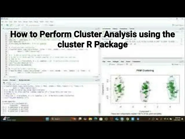
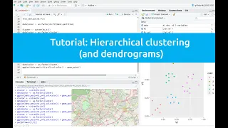
hello yeah in this video um I want to show you how to perform cluster analysis using the cluster package in R okay so there's many cluster analysis packages in our um we showed you how to do class analysis using uh K means and uh H clust function in Basa but if you want to be more sophisticated uh in clust analysis there are specialized packages available in our and one of them is called cluster so this uh package contains many many functions uh it's quite apprehensive okay um I'm not sure I can cover uh each and every s Le detail in this package so I'll try to give a kind of a broad uh view uh for this package um hope you can learn something uh from this video okay so first let's uh just install it and then load it and then we can set random C and then we create a data set uh actually with three clusters from um normal distributions and first um I want to show you how to do a partitioning around mids Pam method so this so-called mids uh they are the initial cluster centers so basically Pam it atively iteratively reduce the total dis dissimilarity there's a measure for that until the cluster stabilized okay that's how it works and uh one strength of Pam is is not sensitive to outliers in the data set uh another strength is the distance uh can be very flexible you can use many different types of distances um so since this is um method in which you have to specify uh the data initial data points uh you have to tell R how many clusters you want to you want to uh use so here is the Pam then data and k equal to three so that's the with tail pan there be three clusters okay and then we can print out uh the mids so basically these are the centers um of the data points and then we can use the class plot function to plot out the Pam clustering so it look like that uh again we cheated when we create the data set uh so make it very easy to uh separate okay so this what this look like you got three clusters there and we got the observation numbers there okay all right the next one is called the Clara or clustering large applications so in our sample data set uh the sample size is not very large so the computation went very fast uh but if we have very large data set then Pam can be very time consuming because where every time we do an iteration we are doing the computation for the entire set okay so um with the data set is very large then we can use Clara uh basically uh cler draws similar a smaller sample size random samples of the larger data set and then run Pam on that random sample and put them together and then then do the iterations and then complete the clustering so the syntax is clear data K 3 samples equal to five okay and then you can print out the mids here um and then you can visualize uh the clustering uh look like very similar uh the three groups um uh and also um you can compute this similarity me uh measures uh and it's called the Goa dis similarity for mixed data uh we did not really talk about the type of data we can use for cluster analysis uh when we generate data we assume they're continuous like for from normal distributions but if you have like both categorical and continuous data uh we call it mixed data and you can use actually the gawa dis cimity um to generate this uh this similarity measures and use that for clustering so we can uh set another random seed and generate a data set with mixed data now you got the continuous and you got a categorical variable then you can use the DAC function uh so the DAC the mixed data matric gawa okay and put them into part a gawa uncore disc and then you can print out the data Matrix look like that okay and then with that um this city Matrix you can feed it to the H clust function uh and you can specify methal the average and then you can flot out the hierarchical clustering using the G similarity okay so you did this hierarchic clustering even if the data are mixed type okay all right and then we have the equative methods in hercal clustering and there are uh here we we're experimenting four types of method single complete average and w. D2 with the mean to methods and then we split the uh graphic window into 2 by two so and we plot out these four um clust heral cluster uh dendrogram um using four different type of um methods okay and reset the layout uh next topic is called the Cy analysis for Pam uh C analysis for assessing the quality of the Clusters okay so it will compute something called the average C whole te width uh when uh this measure close to one it indicates good quality uh if it close to zero that means some there's some overlapping uh and if it's negative then there's some some misclassifying data points okay and also it will generate uh the cell H plot which are basically bar charts of all the data points uh grouped in clusters and um you can also see similar information from the plot okay so let's uh generate that using the cell H function and then we can plot it out it look like that okay so you can see there's three clusters uh in different colors and the bar charts uh so you you you can you can see they're very much close to one the average being 8788 88 so they're pretty good quality clusters in this case okay and we can also um calculate the agative coefficient uh to evaluate the strengths of the hierarchical clustering structure here um when we use um this function uh I found out the method here um so we're using the AG n function uh there's no w. T2 a D2 method so it only the W method so I change the method Vector the the force component into W and then we run that and you can see uh the etive coefficient for all four methods um they are 0.
967 0. 988 0. 981 and 0.