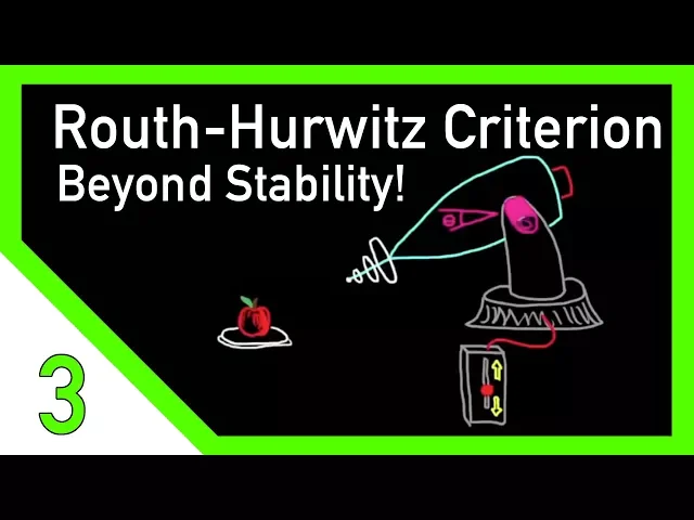
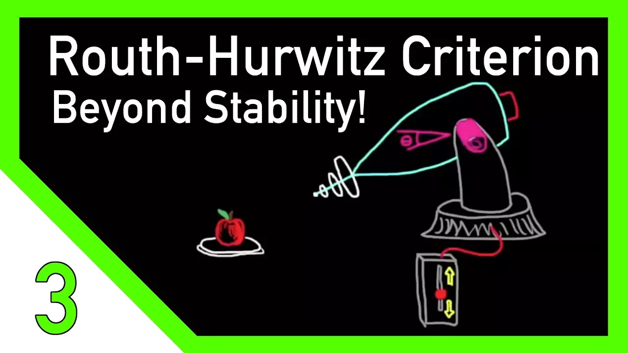
welcome back to control system lectures this is the third and final video covering the basics of the router wits criterion the first two videos describe the method for filling out the route the Ray even under special circumstances and how to use the array to assess system stability in this lecture I want to explain some of the useful ways to use the route the Ray that go beyond just assessing system stability so let's get to it in this example you're working on the next great engineering marvel which in this case is a shrink-ray and this is
mounted on top of a gimbal which can rotate the Ray up and down by an angle theta you have a remote with a joystick that can move up and down to drive the motor in the gimbal to move the Ray and through system tests you determine that the transfer function for the plant looks like this where the joystick is the input and the angle of the Ray theta is the output and this is the open-loop transfer function and you can see that it has the poles explicitly defined in the function when it's written in this
form is really easy to see that the poles in this case are minus 1 minus 2 minus 3 and minus 4 so now you turn on the machine and you try to command it to point towards an apple that's sitting on a table but you realize that you or your slow reflexes aren't good enough to track the angle that you want so you decide that you need to add automatic feedback control and the block diagram would look like this where theta reference is the angle that would cause the ray to point towards the Apple in
order to feedback the angle of the ray you add a resolver to it and for simplicity and remove the dynamics of this sensor by making it one in the feedback path or really what I've done is assume that the sensor is perfect and that it always knows exactly the angle of the ray without delay or error so now you have a computer hooked up to it which is the controller but you're a little nervous that it might go crazy and start shrinking everything so before you turn it on you want to determine the closed-loop stability
and since you're a skilled controls engineer you can do this by reviewing the open-loop transfer function of the plant with a bode plot or a Nyquist plot and these two methods are very popular not only for assessing closed-loop stability but also for determining stability margins so you wouldn't really be wrong in choosing one of these two methods however what if you determine the open-loop transfer function looked something like this where the poles and zeros are not explicitly defined this makes using bode plot very difficult because it's hard to approximate a bode plot by hand without
building up from explicit poles and zeros this also makes the Nyquist plot difficult because although you don't necessarily need to know where the poles and zeros are you still need to know how many exist in the right and left half planes and now as you know the best method for determining closed-loop stability of a system like this is with the router wits criterion but very often you're not just feeding back the output and sending the error signal directly into the plant if you are able to get away with such a simple controller which has a
gain of 1 then great but usually you're trying to tune the gain K of a controller to get the response that you require all while staying stable so the question is now can we use the same techniques with the rath array to determine what range of gains will produce a stable system absolutely let me set up a visual example real quick so you can get an idea of how adjusting the gain changes a system turning the gain is a lot like adjusting the volume of a radio or amplifier when you turn the volume up the
amplitude of the signals get larger and the sound increases and if there is no feedback then you could increase the gain forever in a linear system without a problem but let's say that you're a rock star at a concert and you set up your speaker system behind you in such a way that sound from the speaker could be picked up by the microphone and so now with the volume or the gain around this loop is too large then you're going to start to get unwanted feedback in the system that will distort the sound and possibly
even destroy the instruments so you turn it down to reduce the chances of this happening except that you are a rock star after all and you have an audience that wants to hear loud music so really your goal is to increase the gain large enough to satisfy your audience while keeping the game low enough to keep the system stable and this is a pretty situation in real engineering problems you're trying to increase the gain as large as you can to get the fastest response to satisfy your requirements or the audience but not too high of
gain as to cause the system to go unstable okay let's get back to our example let's see how we can solve this problem using the Roth array I'll rewrite the block diagram from above right here now we want to simplify this block diagram down to a single transfer function for the system let me call the denominator of the plant den of s so that the plant is now 1/10 of s then the simplified block diagram can be written as K divided by den of s divided by 1 plus K over din of s now you
can multiply the top and bottom by den of s to get K divided by den of s plus K and then you can easily see that our new characteristic equation is our old characteristic equation plus the gain K and we can write that as s to the fourth plus s cubed plus 35 s squared plus 50 s plus 24 plus K and now we set up the router ray and we can use the coefficients in this polynomial to fill out the first two rows just like we've done in all of the other problems and then
we can fill out the other rows using the figure 8 method but notice that we're keeping K is a variable throughout this whole process and if I've actually worked this problem out before starting this video maybe I would have noticed that this produces a rather ugly equation at the end here and perhaps I could have simplified it unfortunately this is what the problem produces so we'll just run with it now at this point we can count the number of roots in the right-half plane just as before by Counting the number of sign changes in the
first column and you can see that the first three entries are all positive which means that in order to have a stable system we need to choose K such that the next two entries are also positive this will ensure that there are no sign changes in that first column and it's pretty easy to see what values of K would make the first equation positive and probably not as easy for the second but you can solve both equations and choose the smallest positive value of K that satisfies both of them which in this case K must
be less than 126 notice that what we're doing here is just determining what value of K causes the sign to change in the first column but what this really means is that at that game a pole is on the verge of wandering over from the left half plane to the right half plane and the system is marginally stable you know what the gain margin is which is how much the gain can be increased before the system is unstable in this case it's 126 but you don't actually know where the poles are all that we are
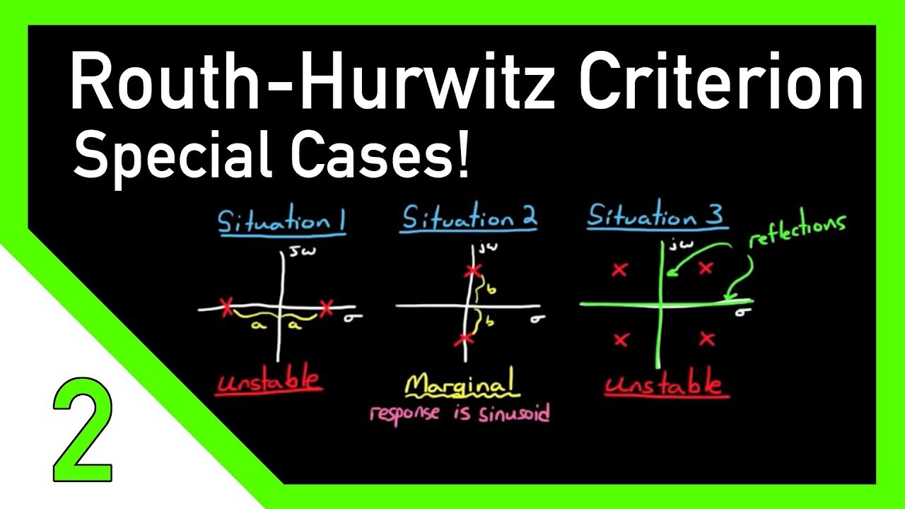
really doing here is increasing the gain in the system and we're monitoring that J Omega line to determine how much gain the system can handle before at least one root goes into the right half plane and crosses over that line but let me take a step back here and mention exactly what it means to have a pole the impulse response of a pole is e to the St when s is real and negative the response decays exponentially and the further from the J Omega axis the faster the response decays because s is a larger real
you and the same goes in the right-half plane as well the further from the J Omega axis the faster the response goes unstable now when s is purely imaginary the response is sinusoidal since E - an imaginary number is a sinusoid and the closer the imaginary roots are to the real axis the slower the frequency and so the slower the oscillations and when there's a mix of the two so that you have both a real and imaginary component then the response decays at the rate associated with the real component and oscillates at the rate associated
with the imaginary component so you can have exponentially decaying and oscillating signals but when we're talking about stability we're only talking about the exponentially decaying or growing term ie the real component and one way to describe how far a pole is from the J Omega axis is by stating the poles time to double or time to half this is the amount of time it takes to half or double the initial signal having a time requirement like this is especially useful when describing systems that interact with humans because you need to ensure that the system is
not too fast or too slow for them to respond to so now the question becomes is there a way to ensure our system meets our time to half requirement using the route array and of course the answer is yes otherwise I wouldn't have asked the question so when you're given a time to half requirement what you're really getting at is that all of the poles in the system must lie to the left of some non-zero line in the left half plane for this example we'll say that this line is at negative one and we'll call
this line the Z line now we can take a polynomial that's written in terms of s and write it in terms of Z by saying that s equals Z minus 1 and visually you can see that this is true because when a pole is right on the Z line it's minus 1 from the S line so now we can take any characteristic equation and substitute Z minus 1 everywhere there's an s after you make the substitution you can expand the polynomial then combine all the like terms and simplify it back into a standard third order
polynomial form and now we can use the router array to determine if this system has any roots to the right of the Z line or in other words if the system has any roots with real components greater than minus 1 and since there are no sign changes in the first column all roots are to the left of s equals minus 1 okay one last thing before in this video I just want to say that in real engineering problems you're gonna rarely if ever use this method but I don't want this fact to discourage you from
really trying to learn and understand it there's because so much of designing a control system is understanding the problem you're trying to solve and really understanding the controls on the most fundamental level for example tuning a controller can result in repeated trial and error attempts if you don't have an intuitive understanding of how adjusting the gain affects your system experience and intuition can play a large part in designing a control system and this is why I'm always pushing for an intuitive understanding of the topics it's not because you will be using these methods every day
on the job it's because they help you grasp the overall picture and ultimately make you a better controls engineer I hope these three videos helped you out with the Ralph Hurwitz criterion and the Roth array as always please leave questions or comments in the space below and I'll do my best to address it and also don't forget to subscribe thanks for watching