in the previous video we have seen what duality means for convex sets and what duality means for convex functions in this video we will see what duality means for convex optimization problems and we will see how it can be helpful for designing efficient algorithms for solving these problems [Music] let's work with an example this time imagine you are the captain of a ship in the middle of the ocean using some sophisticated equipment you know that the rain is coming from some direction c for example c equals the vector 1 1. so you decide to steer
the ship in the opposite direction as much as possible you also remember that the sea is infested with sharks except for a safe circular region of radius one unit this now becomes an optimization problem our decision variable is the two-dimensional vector x that represents the position of the ship our objective is c transpose x or in other words x one plus x and we have a single constraint which is that we need to pick x from the unit disk note that this is a convex optimization problem because the objective function is linear and in particular
convex and the constraint is given by a convex function one thing we would love to do is somehow get rid of the constraint indeed if this constraint did not exist then we would just have an unconstrained convex optimization problem and we have discussed those in detail in the previous video and the nice way to visualize what is going on in that case is to imagine that the level of the c is tilted according to the objective function in such a way that low sea levels correspond to low objective values and high sea levels to high
objective values it becomes visually clear that the answer would simply be to steer the ship in the direction of minus c which matches our intuition so keep this analogy in mind for later because it will be useful but life is unfair and you often need to deal with constraints otherwise you become a snack for some hungry sharks so one way to get rid of a constraint is to move it to the objective function via what is called a penalty function so what is a penalty function you ask well it is simply a function that penalizes
you for not satisfying a constraint and a natural choice for this penalty function is a function that takes the value of 0 when its argument is negative and the value plus infinity when its argument is positive let's call this particular penalty function the zero infinity penalty for later references now if you pick an x that satisfies the constraint then the penalty term will evaluate to zero it is as if the penalty term simply was not there but if you pick an x that does not satisfy the constraint then the penalty term will evaluate to plus
infinity which is really the worst possible outcome you can hope for as far as minimization problems are concerned visually this penalty function raises the sea level outside of our disk of safety to plus infinity so it makes it no longer desirable to steer the shape outside of this circle even if the original objective value was smaller there and this penalty term is almost perfect we generally get rid of the constraint without affecting the optimal value of the minimization problem the price we pay however is that our objective function now can take the value plus infinity
and while we can just replace it with some really large value like a million we would still have the issue that our objective function has become discontinuous and it would no longer make sense to take the gradient of this function for example one thing we could try here is approximate this penalty function with another function that is smooth and does not take infinite values the simplest thing we could try here is to pick a linear function as our penalty function something like u times y where the slope u is a non-negative number visually you can
see how this penalty is a smooth approximation of the zero infinity penalty function how does this linear penalty work well the idea is simple if you pick an x that does not satisfy the constraint this penalty term will evaluate not to infinity this time but to a quantity that is proportional to how much you violated the constraint and if you pick an x that satisfies the constraint believe it or not you actually get rewarded and as much as we like it when we get rewarded for doing the right thing and penalize for violating constraints it
is less than ideal in this scenario because it affects the optimal value of our minimization problem and the amount by which it affects the optimal value depends on the value of the slope you clearly for any value of u this linear approximation is rather poor but notice that if you consider all of the u's and take the maximum of the corresponding linear penalties you can check by looking at the plot that you recover the original zero infinity penalty function which is pretty neat right so let's try to use this maximum as our penalty function and
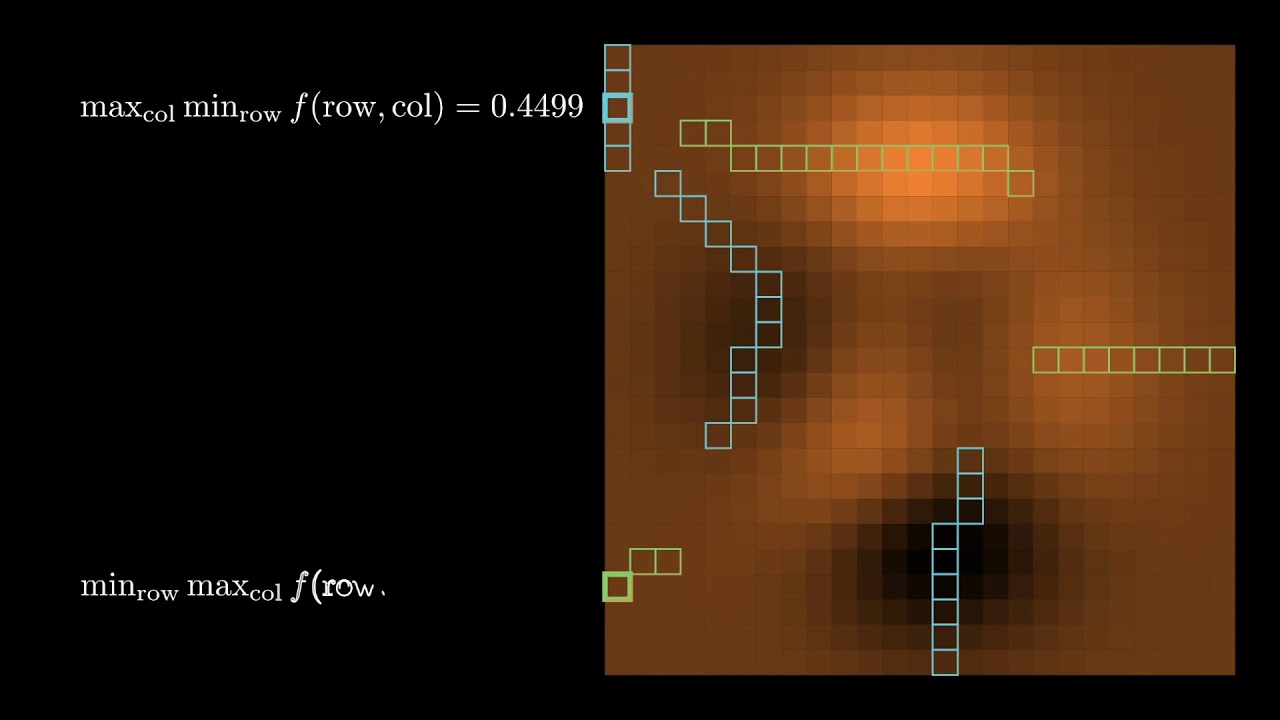
note that now we can take the maximum outside since x1 plus x2 does not depend on you what we have now is what is called a min max problem and a nice interpretation of what's going on here is to view the min max problem as a two persons game we have an x player and a u player the x player picks an x to try to make this quantity small while the u player will try to penalize us if we don't satisfy the constraints and pku that makes this term big [Music] and in games like
these it is important to know who plays first indeed if given the choice you will always want to go second because the second player gets the benefit of knowing what the first player did so here naturally the x player might protest that it is not fair that he always goes first and wonders what happens if the other player you goes first for a change well if you goes first then the x player's job becomes much simpler he just needs to minimize this quantity and i emphasize here that this quantity is a convex function without any
constraints so x can just take the gradient of this quantity set it to 0 and solve for x and now that we know what the response of x should be we can plug that back in maximize with respect to u [Music] and get the solution x 1 equals x 2 equals minus square root of 2 over 2. it is important to note here that what we have just done is not solve the original problem but a variation of it the problem that we solved is actually called the dual problem while the original problem is called
the primal problem and there are a lot of benefits to considering this dual problem but before we talk about that let's just take a step back from this example for a bit and see what the dual problem is for convex optimization problems in general let us now consider a general convex optimization problem and inspired by the example we just saw let's try to derive its dual the first step is to get rid of the constraints for that multiply each function in the constraints with a scalar that represents the slope of our penalty function and move
these functions from the constraints to the objective function and similar to what we did in the example we are going to take the maximum over the scalars uis and vi's for inequality constraints like the ones we had in the example we really want the cost to be positive while for equality constraints where we want to penalize positive and negative values alike we will allow the slope to be positive or negative and now to get the dual problem we pull the maximum outside and we switch the order of the min and the max this quantity here
is known in the literature as the lagrangian of the optimization problem and the dual problem is referred to as the lagrangian du and we will go back to the lagrangian in a second keywords are in order at this point first the dual problem has one variable for each constraint of the primer these can be interpreted as the cost or price for violating that constraint second the dual problem gives us a lower bound on the optimal value of the primal problem this is because in the dual problem and unlike in the primal problem the x player
which tries to make our objective function small goes second and therefore has the advantage and finally and what is more interesting is that under some mild assumptions strong duality holds this means that the optimal value of the primal and the dual problem actually coincide so you can solve whichever you find easiest and you will find the right answer the assumptions i refer to are a bit technical so i won't list them here just know that they are usually satisfied and they are satisfied for our toe example for instance anyway we won't worry too much about
that and we're just going to assume from now on that strong duality holds and now that we have derived the dual problem let's see how it can be useful for solving convex optimization problems and this will lead us to the next theme of this video which is the celebrated kkt conditions let's consider our friend the lagrangian again remember that the x player tries to minimize this quantity so at the optimal solution x the gradient with respect to x better be zero this is a necessary condition that any optimal solution to the optimization problem should satisfy
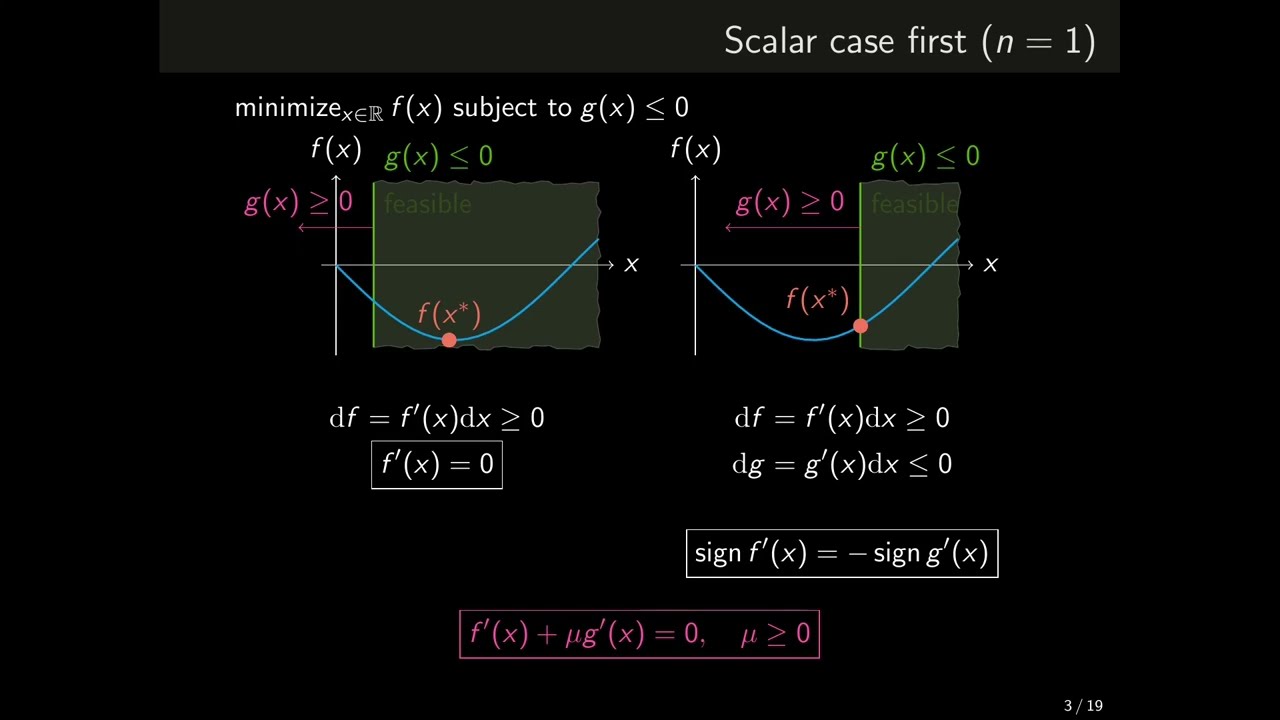
think of it as a generalization of the condition that grad of f equals zero for any minimizer of an unconstrained optimization problem [Music] there is a nice geometric intuition behind this condition and let's see a visual explanation of what is happening here and for simplicity let's consider a case where we have only one inequality just like the example we saw before in which case this condition is saying that grad f and grad g are inversely proportional to each other let us delimit the feasible region given by g with a green line and consider an arbitrary
point x inside this region at this point x let's draw the gradient of g and the gradient of f and remember what gradients represent when you follow the opposite direction to the gradient of a function the value of that function will decrease at least locally so we know that in this green rectangle the value of g will remain smaller than zero and therefore we can safely move x inside of this region without fear of violating the constraint similarly if you nudge x to fall in the yellow region you will reduce and hence improve the objective
function f so if the yellow and green region intersect it means that you can nudge your x a bit stay feasible and improve the objective value so such an x cannot be optimal said differently if x were optimal then necessarily the two regions should not intersect which can only happen if the gradient of f and g are inversely proportional to each other at this point it is a good idea to recap what we have just seen we have seen that if x is an optimal solution then it should satisfy this gradient condition and you might
wonder if this condition is also sufficient in the sense that if for some point x you succeeded in finding a scalar u that makes this condition hold then that makes x an optimal solution after all for unconstrained optimization problems grad f equals 0 guarantees that x is an optimal solution unfortunately it turns out that this implication is not quite true and you need additional assumptions on x and u to make it old on the bright side however these additional assumptions are quite natural and they are as follows first and foremost we need x to be
feasible second the scalar u should be negative and last that the penalty term u times g should be zero only this last condition is new and the meaning of this condition is that at the end of the day if you choose x and u properly the penalty term u times g should not affect the optimal value of our minimization problem and hence should be zero these conditions together are known as the kkt conditions and they are extremely important in convex optimization the big pro of kkt is that you essentially reduce solving an optimization problem to
solving a bunch of equations and inequalities and as you can imagine this is extremely useful for designing general purpose optimization solvers you can try to solve for these conditions by hand for small examples like the one we saw earlier but that easily becomes complicated for more involved problems so we need to develop a more sophisticated machinery and that is exactly where the interior point method comes in [Music] as i said earlier you can view the interior point method as a way to solve the kkkt conditions there are two big insights or solution techniques behind the
interior point method and these techniques are actually useful for a lot of other problems in mathematics beyond just optimization the first insight is that we are not going to solve the kkt conditions exactly but we are going to solve a modified or perturbed version of these conditions that we call kkt of t where t is a positive parameter that controls the degree of this perturbation and while we're at it let's call the solution to these perturbed equations x of t and call the solution to the original equations x star the perturbation works as follows we
keep all of the kkt conditions the same except for the last equation in the right hand side of this equation we replace zero with a negative number minus t hopefully when t is small x of t and x star will be close or in other terms as the perturbation parameter t goes to zero x t converges to x star so far we have talked about how to do this perturbation but not why we do this perturbation in the first place the main reason behind it is that and as we will see now the modified kkt
conditions are much easier to solve if u times g equals minus t then we immediately get the value of u from the value of x as u equals minus t over g of x let's plug this value of u back in the gradient equation as it turns out this quantity is actually the gradient of f minus t of log minus g and you might want to pause the video here and work out the gradient by hand to convince yourselves of this fact now in order to solve this gradient equation we just need to minimize this
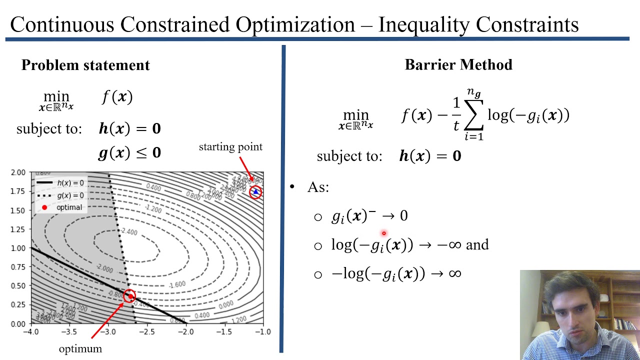
function indeed at the point where the minimum is attained we know that the gradient must be zero and as a bonus note that if you succeed in minimizing this function then the solution that you will find will automatically satisfy the constraint g of x smaller than zero because if g were positive log minus g would be plus infinity and as a bonus of this bonus you will be automatically positive so from now on we are in unconstrained minimization territory and you can use something like newton's method to perform this minimization there is a nice geometric
interpretation behind this minimization problem it is as if the penalty term for violating the constraint was given by the log function and the scalar t controls the degree of this penalty [Music] the issue here is that we want to take t to be as small as possible so that the penalty term doesn't affect our objective value too much but taking t to be too small causes issues as it makes t times log behave like the discontinuous zero infinity penalty function we saw earlier and practically speaking what is going to happen is that newton's method will
be extremely slow to converge and will cause numerical issues the second insight alleviates this issue in a very clever way the second insight is that we don't have to take t to be small right away but start with a big t and make it smaller and smaller let's see why this is a useful strategy if t is a very big number then the log term dominates and it is as if the first term did not exist and because log is increasing this is the same as minimizing g of x which you can do by you
guessed it newton's method in our toy example this step would give the center of the disk and more generally the point you get at this step is called the analytic center of the feasible region once you have a solution for a given t you can try to solve for a slightly smaller t prime say t prime equals 0.9 times t we will again use newton's method but now the difference is that we will specify x of t as a starting point for newton's method the one thing you need to know about newton's method is that
if you initialize it with a point that is close to the optimal solution then it will run super fast and by design we have that x of t is close to x of t prime so by initializing newton from x of t computing x of t prime will be easy and the interior point method will keep iterating and making t smaller and smaller in a similar fashion until a t that is deemed close enough to zero is reached so to recap the two insights we just saw the interior point method when applied to a convex
constraint problem will move constraints to the objective function via a log penalty function multiplied by scalar t it will start with a large t effectively finding the analytic center of the feasible set then it will work its way to t equals 0 by going through the path formed by the x's of t this path is called the central path the central path falls in the interior of the feasible region and this is how the interior point method earned its name and the end of the central path is the solution that is eventually returned by the
interior point method we have now reached the end of this video series to conclude let me say that today we have barely scratched the surface of convex optimization there is a lot more to say about duality and there is a lot more to say about the interior point method but hopefully this video has helped to develop the necessary intuition so that in the future if you read about convex optimization in a wikipedia page or research paper you're not completely lost and if you want to dive deeper into the topic a natural reference i encourage you
to look at is this book by boyd and van der bee that i have used personally for preparing this video and the pdf version of this book is freely available online and as always thank you very much for following along and see you next time