CS 285: Lecture 2, Imitation Learning. Part 1

hi welcome to lecture two of cs285 today we're going to talk about supervised learning of behaviors so let's start with a little bit of terminology and notation so we're going to see a lot of terminology in this lecture denoting policies that we're going to be learning from data and we're not going to talk about reinforcement learning just yet we're going to talk about supervised learning methods for learning policies but we'll get started with a lot of the same terminology that we'll use in the rest of the course so typically if you want to represent your

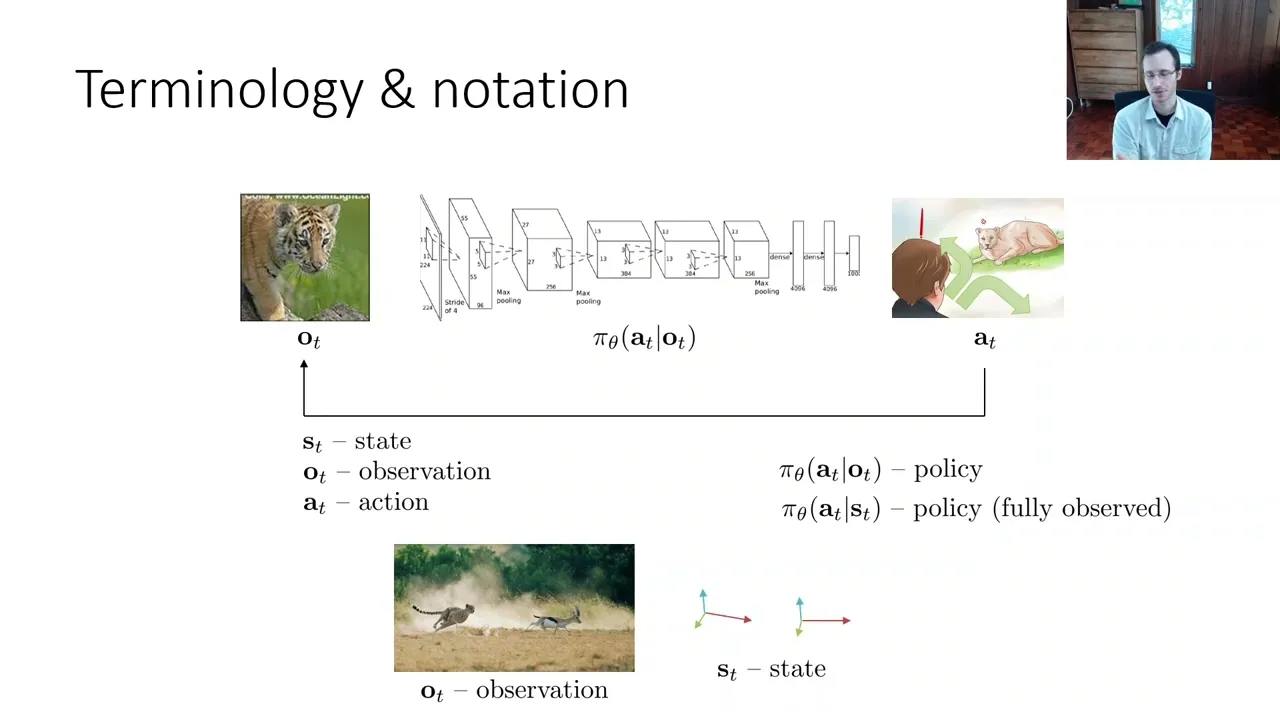
policy you have to represent a mapping from whatever the agent observes to its actions now this is not such a strange object those of you that are familiar with supervised learning you can think of this as much the same way that you represent for example an image classifier an image classifier maps from inputs X to outputs y a policy maps from observations o to outputs a but other than changing the names of the symbols in principle it things haven't actually changed all that much so in the same way that you might train an image classifier

that looks at a picture and outputs the label of that picture you could train a policy that looks at an observation outputs in action same principle we're going to use the letter Pi to denote the policy and the subscript Theta to denote the parameters of that policy which might be for example the weights in a neural network now typically in a control problem in a decision-making problem things exist in the context of a temporal process so at this instant in time I might look at the image from my camera and make a decision about what

to do and then at the next incident time I might see a different image and make a different decision so typically we will write that both the inputs and outputs with a subscript lowercase T to denote the time step t for almost all of the discussion in the score so we're going to operate on discrete time meaning that t you can think of it as an integer that starts with zero and is then incremented with every time step but of course in a in a real physical system T might correspond to some continuous notion of

time for example T equals zero might be zero milliseconds into the Control process T equals one might be 200 milliseconds equals to maybe 400 milliseconds and so on now in an actual sequential decision making process of course the action that you choose will affect the observations that you see in the future and your actions are not going to be image labels like they are for example in the standard image classification task but they're going to be decisions decisions that are bearing on future outcomes so instead of predicting whether the picture is a picture of a

tiger you might predict a choice of action like run away or ignore it or do something else but this doesn't really change the representation of the policy if you have a discrete action space you would still represent the policy and basically the same exact way that you represent an image classifier if your inputs are images you could also have continuous action spaces and in that case perhaps the output would not be a discrete label maybe it would be the parameters of a continuous distribution a very common Choice here is to represent the distribution over a

as a gaussian distribution which means that the policy would output the mean and the covariance for that gaussian but there are many other choices we could make so to recap our terminology we're going to have observations which we denote with the letter O and the subscript T to denote that it's the observation of time t our output will be actions which we denote with the letter a and a subscript t and our goal will be to learn policies that in the most General sense are going to be distributions over a given o now something I

want to note here because this is sometimes a source of confusion a policy needs to provide us with an action to take in the most General case policies are distributions meaning that they assign a probability to all the possible actions uh given a particular observation of course a policy could be deterministic meaning that it prescribes a single action for a given observation that's a special case of a distribution it's just a distribution that assigns a probability of one to something and a probability of zero to everything else so in most uh cases we will actually

talk about stochastic policies policies that have specified distribution over actions but keep in mind this is fully General in the sense that deterministic policies are simply a special case of these distributions and it's very convenient to talk about distributions here for the same reason that we tend to talk about distributions and supervised learning so in supervised learning interclassifying images perhaps you only really want to predict one label for a given image but you might still learn distribution over labels and then just take the most likely output and that makes training these things a lot more

convenient and it's the same way with decision making and control that training these policies as probability distributions often is much more convenient even if in the end we only want the single best action now one more term that we have to introduce and here we're going to start getting to some of the idiosyncrasies of sequential decision making is the notion of a state the state is going to be denoted with the letter S and also the subscript t and a state is in general a distinct thing from the observation understanding this distinction will be very

important for certain types of reinforcement learning algorithms it's not so important for today's lecture because for imitation learning we often don't need to make this distinction although even here it'll be important when we try to understand the theoretical underpinnings of some of these imitation learning methods and sometimes when we learn policies we'll write policies as distributions over a given s rather than given o I will try to point out when this is happening and why but to understand the difference between these two objects let's talk about the difference between states and observations and then we'll

come back to this and typically we'll we'll refer to policies that are conditioned on a full State as fully observed policies as opposed to policies conditional observation which might have only personal information so what I mean by this well let's say that you are observing a picture of a cheetah chasing a gazelle and you need to make some decision about what to do in this situation now the picture consists of pixels so they're recordings from a camera you know that underneath those pixels there are actual physical events taking place that you know maybe the cheetah

has a position and velocity and so does the gazelle but the input technically is just an array of pixels so that's the observation the state is what produced that observation and the state is a concise and complete physical description of the world so if you knew the positions and velocities and maybe like the mental state of the cheetah and the gazelle you could figure out what they're going to do next the observation sometimes contains everything you need to infer the state but not necessarily so for example maybe there's a car driving in front and you

don't see the cheetah the cheetah is still there the state hasn't changed just because it's not visible but the observation might have changed so in general it might not be possible to perfectly infer the current state St from the current observation OT whereas going the other way going from st2ot by definition of what a state is is always possible because a state always encodes all the information you need to produce the observation so if it would help to think about it this way if you imagine this was a simulation St might be the entire state

of the computer's memory encoding a full state of the simulator whereas the observation is just an image that is rendered out based on that state on the computer screen so going from observation back to State might not be possible if some things are not visible now if we want to make this a little bit more precise and we can we can describe this in the language of probabilistic graphical models so in the language of probabilistic graphical models we can draw a graphical model that represents the relationship between states observations and actions for those of you

that took some course that covers Bayes Nets this will look familiar for those of you that haven't roughly speaking in these pictures the edges denote conditional Independence relationships so if there's an edge then the variable is not independent of its parents and in some cases these things can encode independencies I won't get into the details of how to understand probabilistographical models if you haven't covered this part this won't entirely make sense to you but hopefully the verbal explanation of the relationship between these variables will still make sense so the policy Pi Theta is at least

for the partial observed case a relationship between o and a so it gives the conditional distribution over a given o so that's this Edge in the graph the state is what determines how you transition to the next state so the state and action together provide a probability distribution over the next state P of St plus one given s t a t that is sometimes referred as the transition probabilities or the Dynamics you can think of this as basically the physics of the underlying world so when we write down equations of motion and physics we don't

write down equations describing how image pixels move around we write down equations about how rigid bodies move and things like that so that's referring to S the state the position of the velocity of the cheetah so the cheetah might transition to a different position based on its current velocity and maybe based on how hungry the cheetah is and what it's trying to do and that's all captured in the state and then uh something to note about the state is that the state S3 here is conditionally independent of the state S1 if you know the state

S2 so let me say that again because that might have been a little bit unclear if you know the state S2 and you need to figure out the state S3 then S1 doesn't give you any additional information that means that S3 is conditionally dependent of S1 given S2 this is what is referred to as the Markov property and it's one of the most fundamental defining features of a state essentially if you know the state now then the state in the past does not matter to you because you know everything about the state of the world

and that actually makes sense if you think back to that that analogy about the computer simulator if you know the full state of the memory of the computer that's all you really need to put in order to predict future States because the past memory of the computer doesn't matter the computer is only going to be making its simulation stuff based on what's In memory now the computer itself has no access to its memory in the past only its memory now so it makes sense that the future is independent of the past given the present so

this is referred to as the Markov property and it's very very important the Markov property essentially defines what it means to be a state a state is that which captures everything you need to know to predict the future without knowing the past that doesn't mean that the future is perfectly predictable the future might still be random there might be stochasticity but knowing the past doesn't help you resolve that randomness okay so just to finish this uh discussion now it's hopefully clear with the distinction between policies that operate on observations Pi of a t given OT

and policies that operate on States but I have 80 given stns so some algorithms especially some of the later reinforced learning algorithms will describe can only learn policies that operate on States meaning that they require the input into the policy to satisfy the Markov property to fully encode the entire cellular system some policies some algorithms will not require this some algorithms will be perfectly happy to operate on partial observations that are perhaps insufficient to infer the state I'll try to make this distinction every time I present an algorithm but I will warn you right now

that a reinforcement learning practitioners and researchers have a very bad habit of often confounding o and S so sometimes people will refer to O as s they'll say oh I this is my state when in fact they mean this is my observation sometimes vice versa and sometimes I'll make this distinction very unclear sometimes they'll switch back and forth between observations in the states so this confusion often happens if everything is going well this confusion is benign because it's typically this kind of confusion typically happens for algorithms where it doesn't matter whether it's state or observation

so then it's kind of okay to mix them I'll try not to mix them but sometimes I'll fall into old habits and mix them anyway in which case I'll do my best to tell you but be warned that ons gets mixed up a lot if you want to be fully reversed and fully correct this slide explains the difference so as an asylum notation in this class we use the standard reinforcement learning notation where s denotes States and a denotes actions this kind of terminology goes back to the study of dynamic programming which was pioneered in

the 50s and 60s uh principally in the United States by folks Like Richard Bellman and I believe the sna notation is actually was first used in his work although I could be wrong about that those of you that have more of a controls or robotics background might be familiar with a different notation which means exactly the same thing so if you've seen the symbol X used to denote State such as a configuration of a robot or a control system and the symbol U to denote the action don't be concerned it means exactly the same thing

this kind of notation is uh more commonly used in controls a lot of it goes back to the study of optimal control and optimization much of which was actually pioneered in the Soviet Union by Volkswagen and much like the word action begins with symbol a the word action also begins with a symbol uh in Russian so that's why we have u x well because it's a commonly used variable in algebra okay so that's the set now let's actually talk about imitation the main topic of today's discussion so our goal will be to learn policies which

are distributions over a given o and to do this using supervised learning algorithms so since uh getting data of people running away from Tigers is not something that you can do very readily I'm going to use a different running example throughout today's lecture which is a kind of autonomous driving example so our observations will be images from a dashboard mounted camera on a vehicle and our actions will be steering commands turning left or turning right and you could imagine collecting data by having humans drive cars record their steering wheel commands and record images from their

camera and use this to create a data set so every single time step your camera records an image and you record the steering wheel angle and you create a training tube a lot of this an input o and an output a and you collect this into a training set where A's are labels and O's are inputs and now you can use this training set the same way that you use a labeled data set in let's say image classification and just train a deep neural network to predict distributions over a given o using supervised learning that

is the essence of the most basic kind of imitation learning method we sometimes call this kind of algorithm behavioral cloning because we're attempting to clone the behavior of the human demonstrator so that's a very basic algorithm now from what I've told you just now you can already Implement a basic method for learning policies and what we'll discuss for the rest of today's lecture is does this method work why does it work and when how can we make it work more often and can we develop better algorithms that are a little smarter than just straight up

using supervised learning that will work more consistently so supervised learning produces this policy just like supervised learning might produce an image classifier this is called behavioral clone now these kinds of methods have been around for a very very long time one of the first uh what we call large scale large or larger scale learning based control methods was actually an imitational learning method called Alvin developed in 1989 which stands for autonomous land vehicle in a neural network and that was what would they call a deep RL method for learning based control it used data from

Human drivers to train a neural network with a whole heaping load of hidden units five hole hidden units to look at a 30 by 32 observation of a road and output commands to drive a vehicle and it could drive on roads it could follow lanes and could do some basic stuff you know probably wouldn't be able to handle traffic laws very well but it was a very rough schedule autonomous driving system quite a long time ago but if we want to ask more precisely whether using these behavioral cloning methods in general is guaranteed to work

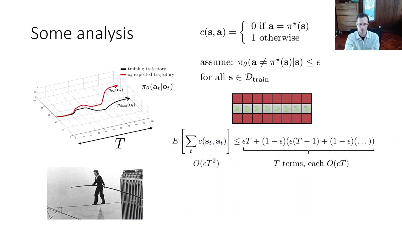
the answer unfortunately is no I will describe we'll discuss the formal reasons for this in a lot more detail but to give you a little bit of intuition to get us started let's think about it like this I'll draw a lot of plots of this sort in today's lecture in these plots uh one of the axes represents the state so imagine the state is one dimensional of course in reality the state is not really one-dimensional but for visualization that's what it's going to be and the other axis is time now in this kind of state

time diagram you can think of this black curvy line as one of the training trajectories in reality of course you would have many training trajectories but for now let's say you have just one and now let's imagine that you train on this training trajectory you get your policy and then you're going to run your policy from the same initial state okay so the red Curve will represent the execution of that policy and let's say you did a really good job so you took all of your lessons from uh cs189 and you took care to make

sure that you're not overfitting and you're not underfitting but of course your policy will still make at least a small mistake right every learn model is not perfect it'll make tiny mistakes even uh in states that are very similar to ones that were seen in training and the problem is that when it makes those tiny mistakes it'll go into states that are different from the ones that saw in training so if the training date involves driving quite straight on the road in the middle of the lane and this makes this policy makes a little deviation

goes a little bit off center now it's seeing something unfamiliar that's a little different than what I saw before and when it sees something that's a little different it's more likely to make a slightly bigger mistake and the re the amount by which these mistakes increase might be very small at first but each additional mistake puts you in a state that's more and more unfamiliar which means that the magnitude of the mistake will increase and that means that by the end if you have a very long trajectory you might be an extremely unfamiliar States and

therefore you might be making extremely large mistakes this doesn't happen in supervised learning in regular supervised learning and the reason it doesn't happen is actually something that we discussed in lecture one there's a particular assumption that we make in supervised learning some of you might remember if you think you might remember it maybe you can pause this video and think about this a little bit then when you on pause I'll tell you the answer the answer of course is the IID property in regular supervised learning we assume that each training point doesn't affect the other

training points which means the label you output for example number one has no bearing on the correct solution for example number two but of course that's not the case here because here when you select an action it actually changes the observation that you will observe at the next time step so it's violating a fairly fundamental assumption that is always assuming regular supervised learning however in reality naive behavioral cloning methods can actually work pretty well these are some results from a fairly old paper at this point from Nvidia where they attempted a behavioral cloning approach for

autonomous driving a kind of modernized version of album and initially they had a lot of trouble that their car was giving them a lot of bad turns running into traffic cones Etc but after they collected a lot of training data 3000 miles of training data they could actually get a vehicle that would follow Lanes reasonably competently uh it could drive around the cones it could follow roads and they always have a safety driver in there and it's not by any means a complete autonomous driving system but it certainly seems like the pessimistic picture on the

previous slide might not actually hold uh in practice at least not always so what is it that this paper actually did what is it that made it work well there are a lot of complex decisions in any machine Learning System but one decision that I wanted to tell you about a little bit that maybe kind of sets the tone for some of the ideas that I'll discuss in the rest of the lecture is a diagram that's buried deeper down in that paper that shows that well okay so they've got their uh recorded steering angle they've

got some convolutional neural net that's pretty typical and they have some cameras but they have this Center camera left camera and right camera and this random shift and rotation what's up with that well there's a little detail on how the policy is trained in that work and the details this so their car actually has three cameras it has a regular forward pacing camera which is the one that's actually going to be driving the car and then they also have a left-facing camera and they take the images from the left facing camera and they label them

not with the steering command that the human actually executed during data collection with a modified steering command that steers a little bit to the right so imagine what that camera sees what the camera sees when the car is driving straight on the road is an image similar to what the car would have seen if it swerved to the left and they synthetically label that with an action that corrects and soars back to the right and they do the same thing for the right facing camera they label it with an action that's a little bit to

the left of the one that the human driver actually used and you can kind of imagine how this might correct some of the issues that I discussed before because if the policy makes a little mistake and it drives a little further to the left than it should have now it's going to see something similar to what that left facing camera would have seen and now that state is not so unfamiliar because it has been seen before in those left-facing cameras now it's being seen in the front-facing camera but the policy doesn't know which camera is

looking through it just knows that it's similar to that image before that was labeled with a turn to the right so it will correct Okay so why did I want to tell you this what's the moral of the story and what does that tell us about how we can actually make naive behavioral cloning methods work pretty well in practice well the moral of the story is that imitation learning via behavioral cloning is not in general guaranteed to work and we'll make this actually precise and we'll describe precisely uh how bad the problem really is and

this is different from supervised learning so for supervised learning you can derive various sample complexity and correctness bounds of course when deep neural Nets are in the picture those bounds often make strong assumptions that might not hold in practice but at least that's a fairly well understood area and this generally doesn't hold them here for a point and the reason fundamentally is the ID assumption the fact that individual outputs will influence future inputs in the sequential setting but they will not in the classic supervised learning setting we can formalize y with a bit of theory

and we'll talk about that today and we can address the problem in a few ways first we can be smart about how we collect and augment our data and that is what that paper from Nvidia did arguably with a technique similar to data augmentation where instead of Simply directly using the true observations that the human driver observed together with their actions they add some additional kind of fake observations from these left and right facing cameras with synthetically altered actions to fix up the problem we can also use very powerful models that make very few mistakes

remember that the issue originally was due to the fact that we made those small mistakes in the beginning which then build up over time if we can minimize the mistakes if we use very powerful models perhaps in combination with the first bullet point then we can mitigate the issue as well there are some other solutions that are maybe a little bit more exotic but can be very useful in some cases for instance sometimes switching to more of a multitask learning formulation learning multiple tasks at the same time can perhaps surprisingly actually make it easier to

perform mutation learning and then we can also change the algorithm we can use a more sophisticated algorithm that directly solves this problem this compounding errors problem and we'll discuss one such algorithm called dagger now that typically involves changing the learning process in the case of dagger it actually changes how the data is collected but it can provide a more principled solution to these issues and you will actually implement this algorithm in your homework so that's what I'll discuss next for the rest of the lecture and the first part will be a discussion of the theory

in part two