Lecture 3 - Damped and Driven Harmonic Oscillator

presented by Caltech so we're doing simple harmonic motion over mass on the spring that we analyzed already I have over here another one if you look at the screen up there you see that that motion looks quite a bit like that motion pretty much the same thing except that what's going on over there is just something that's greater log on a circle you just seeing that peg through a slip there so this I think is a nice illustration of how sines and cosines come into play the motion can look linear but they can still be

underlying sines and cosines governing it so I just thought that was a cute little demonstration and I will try to turn everything off now and remember where I have to go next a lot of buttons to push I don't want to do that yet okay so let's go back to this we saw it did slow down some so there's something going on that's kind of affecting this that's not a perfect simple harmonic oscillator Energy's not completely conserved there's some air resistance presumably there's maybe some friction with the track that we haven't managed to get rid

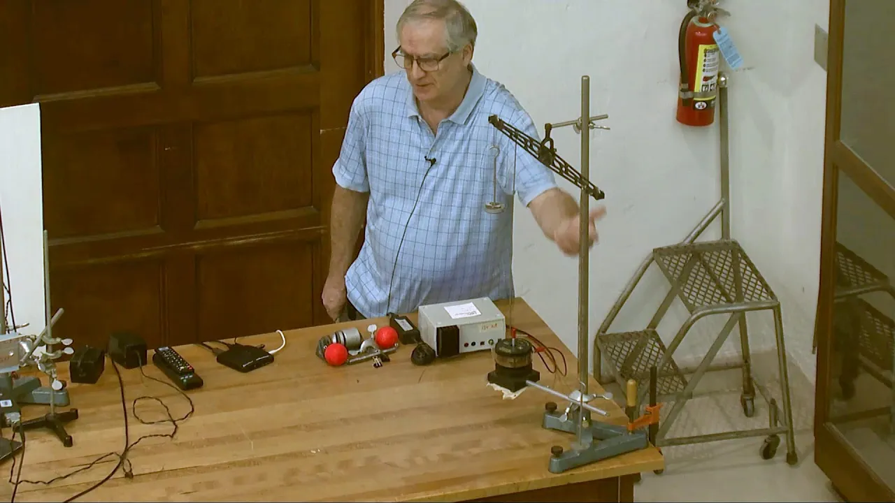
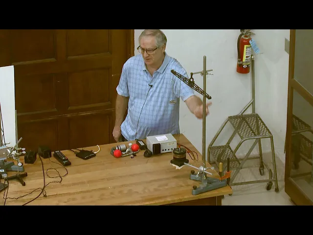
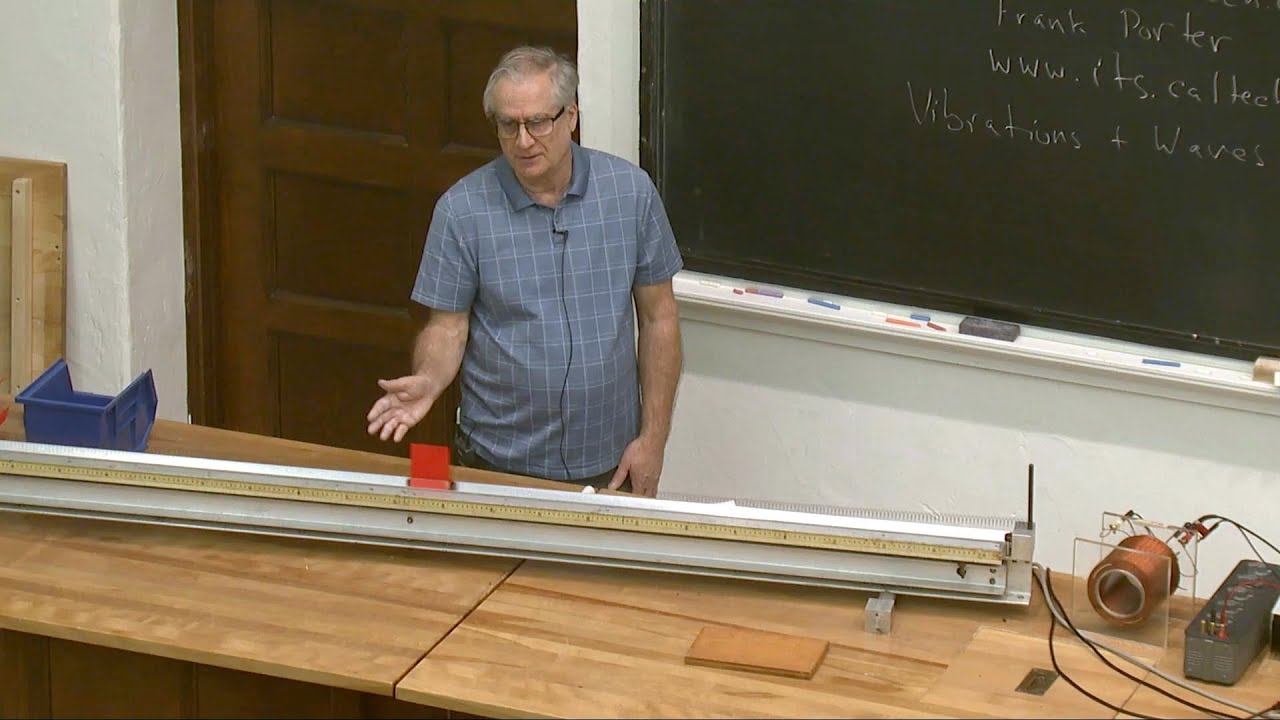
of with even with the levitation it may not be perfect the springs themselves may have some friction in them all contributing to this thing slowing down but we can actually make it worse so just kind of watch how fast how much it's going and then slows down a lot faster and all I did was I put this aluminum bar closer to it this is just a piece of aluminum here I didn't touch it I put it closer but the reason this nut is on the this belt is on this side is because it's holding two

magnets on this side so this has a couple of rather strong magnets such that if I put them close enough to this aluminum bar it slows it down why aluminum is not magnetic what's going on here it really is a pronounced effect so I hope you remember from last year about eddy currents or if you didn't let me tell you about Eddy credits we're dipping our emotions any currents they all we put we put a magnet here and if we put it a little bit of bond and why does that slow it down well it

slows it down because if you put so a little bar is a good conductor it has lots of electrons that are free to move about and we'll put it in the presence of a moving magnetic field or by some Galilean transformation we're putting the magnet in the presence of moving charges either way we have a Lorentz force this is the Lorentz force law so with e equal to zero we have a magnet we have relative motion between the charge and the magnet which is V the velocity of this thing and so that gives a force

on the charges so the force on these charges in this bar are going to make the electrons move and so the electrons move under a force that's proportional to the velocity and when these electrons move of the aluminum it's not a superconductor it's a regular conductor it's a very good conductor but it's not a perfect conductor they're going to dissipate energy in the resistance of the bar and so I am extracting energy from this mechanical system into heat heating up the bar and that's what's causing the damping it's just eddy currents so let me pursue

that a little bit we had a force that's proportional to the velocity in magnitude I mean the force is actually perpendicular to a velocity so it makes these you know makes the motion of these electrons in the bar be a little more complicated but nonetheless the energy eventually goes into heating up the bar the force on the mass is proportional however to you know because the force on the charge has got an equal and opposite reaction in the force on the mass and and so that's forces proportion for the velocity and so somehow the the

effective damping is is looks like it has a force proportional to the velocity so our original equation that says MX double dot equals minus K times X fixed is a function of time that's an additional force term so this is a force equation which is a velocity dependent force which is resisting the motion so it's a restoring force so we can write our force equation as MX double dot is equal to minus K times X minus a velocity dependent restoring force so I'll write this as a function of X dot of course X dot as

a function of time so it's ultimately a function of time with our velocity dependent force zero velocity is equal to zero this Lorentz force is equal to zero of V is equal to 0 and E is equal to zero ok ok and so we anticipate here if I'm just thinking about where this force comes from that their non velocity dependent force is at least to a good approximation proportional to the velocity so we can actually expect that this could be maybe a common theme that other velocity-dependent forces here a resistance and resistance for small enough

motion is his proportion to the velocity if I had a dashpot with you know some configuration was filled with oil for slow enough motion that is for viscous motion the force would be proportional to the velocity of course at higher velocities that your resistance tends to go like V squared but in fact it's a it's a complicated function but we can extract a common theme for small enough motion again using the Taylor series again and let's see how that works let's go over here first so if we consider a velocity dependent force it depends on

the velocity X dot if we make a Taylor series as the force evaluated at zero velocity not X plus X dot times the derivative of the force with respect to X dot evaluated at zero velocity so for small so we're doing the expansion about zero velocity that's what we're doing with our Taylor series expansion so in general I would have an X dot minus the point where expanding about what we're spending about zero plus Oh high order terms in general and so forth so Taylor series expansion I did add a page with a note about

Taylor series expansions to my last week I think I put it with my last week's lectures which I think are posted so let's say so if there's zero force at zero velocity this first term goes away the second term is presumably likely to be nonzero and in this case we have an argument for why it's nonzero and this term goes like the velocity squared so if the velocity smell the velocity squared term is expected normally to be small compared with the velocity term you know things may not happen quite that way in particular instances but

at least in this instance we think that's probably right and in fact in many cases it's an excellent approximation of course if I had just done this [Music] Ravel puzzle we did it let's try that again oh let's say there's another valve back there but I can't reach it can you tell the turn off the compressor do this turn off the compressor there's a leak in the valve oh yeah it does that every now and then oh okay I fit over the valve quite a bit so yeah that's what I couldn't reach that's interesting so

just a relief valve going off okay okay anyway thanks so okay we got it off now that's what I wanted so now the damping force is pretty much all friction and it's kind of behaving funny so when we have a frictional case like this then we need to do a little more analysis things are not quite behaving the way I'm claiming here even as the velocity goes to zero we'll have a lot of force there that's keeping it from moving so we'll probably investigate that a little bit in the homework it's it's a very current

case that doesn't fit the the usual narrative of this course and of course is like this everywhere but it's it's it's useful to keep it in mind that there are some exceptions to the rule so let's continue with the narrative that works in many cases but not always [Applause] so let's see so it's the most ordered in V or X dot we have the lowest nonzero order so because that's the lowest order is that but that's 0 F of V of X dot is something like gamma X dot well I put this M in it's

just a constant times X dot just linear in the in the velocity but I'll put this M in for convenience and the convenience is to is to give this guy units of 1 over time that is it's like has the same units as my frequency does and so this is often an excellent approximation except proof that little issue there we could also consider other situations just to see that it is in fact a little more general with what I've Illustrated here we can consider an LCR circuit and electronics let's see so let's make a circuit

so I've got a circuit with a capacitor resistor and an inductor and I'm considering charged their charge on the capacitor and whatever current we get out of that so let's see we know that the voltage on the abductor is just L di by DT that is L Q double dot the voltage on the capacitor sorry voltage on the capacitor Q equals C times V so that's just you divided by the capacitance the voltage on the resistor is just Ohm's law which is Q dot times R Q dot it's just I Q is like X here

Q is my variable that's going through the sinusoidal variation Q dot is then like the velocity and so we have a voltage a restoring force if you like that's proportional to the analog of the velocity so this will be exactly analogous to this with forces becoming voltages well it's called electro-motive force and position be replaced by the charge so we can try playing with that [Music] yes [Music] see something there do the same thing there I hope maybe ready till oh I go do that and then that too many buttons okay and we just see

a scope trace yeah because everything's off so I have my capacitor my inductor and I can adjust resistors there's already some resistance in this inductor so I turn on my square wave so the red is the voltage across the capacitor so that's the direct analog of position so that's Q basically I mean that's R so I'm just looking at the book this voltage which is just basically Q there's a proportionality factor of C the the yellow curve is the voltage across the inductor and one thing we can see is that when is that these Vantage's

are out of phase quite out of phase that's that's this business of things sloshing back and forth between the two but the yen was a little more complicated because the yellow is basically Q double dot of course if you take a sign and you take a double dot of that you get minus a sign so that makes sense but I want to focus mostly on the red one the voltage across the capacitor we see it's damping out you know it's decreasing from from where it was even though have zero resistance in here that's just because

there's resistance on the end but I can add some additional resistance and you can see what happens so I've added 500 ohms there fifteen hundred ohms 2500 3500 so so the so you still see some oscillation so just look at the red the yellow is complicated because it's cued mo da and we have a source actually here with it's that square wave so it's responding to the Vale the immediate change in the voltage there and and that's not the regime I want to look at it's looking at something else I want to just look at

the at the smooth response and you can see that if I turn this high enough the red curve no longer oscillates it just starts at some voltage and then asymptotically just decreases to zero that words at the bottom is zero okay and I can turn it back on and see the sine wave again I can see it go to zero and and and I can even go farther it just gets a longer and longer kind of tail as I increase the resistance farther here so you can think in terms of time constants in a lot

of time classes okay so we're going to think about that some too so what is going to be the equation that's going to govern this so let's go back to the damp spring although I assert I could write down exactly the same equation just with redefining symbols a little bit for this LCR circuit that I just for the voltage across the capacitor say or the charge on the capacitor so we have M times X double dot so from Newton's law equals minus KX minus gamma M X dot where I've now put in the force from

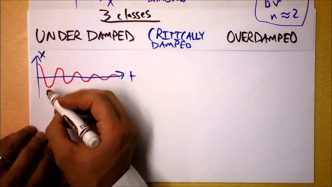
the damping or I can write this as X double dot plus gamma X dot plus Omega naught squared X is equal to zero so with general zero we'd recover our earlier equation what is this well still a second order linear different homogeneous differential equation second order linear homogeneous differential equation just like it was without the game of the Irish we've just added a term proportion to the velocity so what's the solution to that equation going to look like well we've already seen I mean we still lose there's a graph of the solution okay so as

a function of time we expect X to be well what so X is a function time some initial condition maybe up here and there's some sinusoidal variation it dies out with time [Applause] and maybe it goes out with time so let's get it so if I draw an envelope through the piece through the piece of this we see well you know maybe it's some kind of exponential decay and so maybe we have an exponential times the sinusoid it's kind of what it looks like what's the frequency of this well we have a well-defined frequency in

this thing that's our natural frequency of the oscillator which is by definition K over m is not the frequency no it's a good first guess but it's not quite the same system as we does without the damping so who knows we have to figure out let's complicate the issue now let's do something else it's maybe a little boring to just y'all push the push the push this aside and you know I can't roll all oh it's really off now okay fortunately I've got a back-up plan so I have another mass on a spring here okay

it's under gravity but today you know that's same equations of motion and I've got basically a speaker coil that drives it so okay so we can get some motion there so this driving is very small amplitude driving here you see it but it's it's moving up and down according to a sinusoid and you can see the motion of that of the mass of a spring is actually quite a bit bigger than this motion so somehow it's getting amplified let's see I could go ah because if I go very fast so this is hard to tell

it's moving and the mass is not not really moving so if I go really fast it doesn't look like it's moving at all no I know why that wasn't working but you still can't see anything yeah you can you can kind of feel this movie what the mass is basically not moving so if I go really fast with my driving force it's basically not moving let me go and if I go really slow just got some motion here from the shovel is the transient motion is to do power so now it's going to slow to

be able to tell it's moving well let's go to where we can see things happening I'm getting tired of not seeing anything happened so this is very close to one Hertz here and no emotions pretty big and the limit of zero frequency that will move just like this moves it'll be like it's just attached to it and following it and then living a very high frequency this is moving so fast that the spring just doesn't have time to respond and again the amplitude will go to zero but here I'm in a region where I'd kind

of tuned to Omega nought and so it's it's got very large oscillations and I I have some air I could show you that on that as well we can maybe see it on this too okay so like it so right now this is a hundred Hertz is that so I can increase the frequency we go to their 200 so look look at the look at the red curve always clipping yeah look at the red curve let me see look at the red curve [Music] that's not supposed to happen [Music] let's see this thing is doing

bad things to me okay we got a square wave back I really can't show over this the problem is staying on the same scale there's a funny behavior and so the red curve is actually the difference between two different rules just and it's not doing what I wanted it to do then I'll come back to it next time okay I'll figure what's wrong let's just try to solve for the motion so what I want to do is complicate the problem so I'm gonna put a driving force on I'm gonna put a force that's a function

of time this say has that face okay well I know what I did wrong I can show it to you I wanted to show you a driving force right I want a driving force that looks like this so the green is the driving force now I've got a sine wave instead of a square wave so now I can change the frequency which starting to get big you know I started okay so forget that but then it starts that's because the grid is the difference of two voltages somehow and it's it's it's a it's clipping but

it really does a funny thing it's because y'all it's a digital effect I wanted to get let me go to a lower frequency so I can tell what I'm doing don't never get back to where I was there we go now we're back okay thing I should have told you to look at the yellow one but so you can see that if I adjust the scales so this is so pretty low frequency I'll make even flatter you know not much is happening for a while but as I increase the frequency you can certainly see the

yellow the yellow ones getting big and then all of a sudden the red one goes haywire too it's got a digital effect in there that's unfortunate but no I think has some features I don't like you that clearly should have practiced this a little bit more well you saw them you saw the effect if as I will never the frequency the voltage started those started to blow up you can see it best on the yellow the red doesn't work there well I'm not gonna waste your time up okay so what's going to happen here our

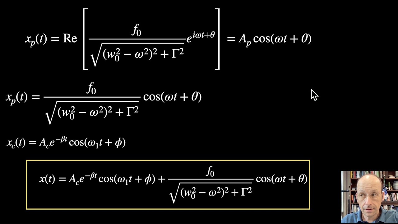
differential equation becomes becomes this of course this Omega is anything we choose I was able to dial it here it has nothing to do with Omega naught where if you like a Nara is here I've just taken this F naught and divided it by m to get rid of the ends here okay so we expect that the motion is going to be oscillatory yeah I mean that looks awesome Ettore what frequency well since the driving force is that frequency Omega after we'd let the damping do its work and all the transient motion dying down is

probably going to be in omega because that's the only frequency that's that's in there for for a long times and the question is is that right so let's try to solve for this motion so the general solution is just a second order now in homogeneous differential equation linear still the general solution will be the general solution to the homogeneous problem so if you find the general solution to this homogeneous problem and then you add to that we take the force-free problem and then you a particular solution to the inhomogeneous problem so that's a general strategy

for solving these differential equations there'll be two integration constants because it's the second-order differential equation and these will be fixed by the boundary conditions or for the initial conditions boundary conditions okay so let's carry out this exercise let's start with a homogeneous equation x double-dot plus gamma X dot plus Omega naught squared X is equal to zero what we do well we have the kind of a guess for the solution we have that as a guess it's maybe an exponential times a sinusoid but we can write sines and cosines as Exponential's to e to the

i-x is just cosine X plus I sine X so maybe just try just try an exponential to this try an exponential solution sort of I mean of course the point here is that you know we don't necessarily have to do anything fancy if we can guess the solution so let's in this case we probably can so let's try X of T is equal to e to some constant times time so let's say so we need to get X dot X dot is a times X X double dot is a squared times X and so let's

plug that into the differential equation we can divide out the X and we get a squared plus gamma plus Omega naught square is equal to zero so okay that's just a quadratic equation in a so that means that a is equal to minus gamma over 2 plus or minus the square root of the M over 2 squared minus Omega naught squared I've already divided by 2 and and so this is my two linearly independent solutions unless Omega naught is equal to gamma over 2 and which chase that zero and something's going down there okay that

I have to worry about well anyway let's point ahead for the moment let's define Omega 1 squared to be Omega naught squared minus gamma squared over 4 thinking about what's inside the bracket which has frequency units and so then a is equal to minus gamma over 2 plus or minus I times Omega 1 as you see I put the minus sign the other way on here so that's looking like if I take this you know I'm going to take e to the 80 so I'm going to get a term that's a damping kind of term

that's exponentially falling and then with this piece I'm going to get something if Omega 1 is a real number is oscillatory no that's kind of looking promising it's kind of what I want okay we've introduced complex numbers here so e to the 80 may be complex we understand here that we'll go take the real part if that happens we're going to take the real part of our solution to get the physical position in fact we don't even have to think about it because that is going to get enforced by our boundary conditions which are going

to be real so we don't actually have to think too hard we will get a real answer once we put in the boundary conditions as long as the boundary conditions are real so let's see solution we have a solution X of T is equal to e to the minus gamma T over 2 times AE to the I Omega 1 T plus B e to the minus I Omega 1t we already see that the oscillation isn't quite at Omega naught its shifted in fact it's shifted lower in frequency then then the natural frequency the damping is

dragging on the system is kind of how you look at that it's kind of trying to resist the motion it's slower it's slowing the frequency down okay but we do have this case that we've got to worry about Omega nought equals M over two implies Omega 1 equal zero one solution we just lost a solution we lost a degree of freedom in our solution space so what we do well it means that something we did here doesn't cover this case quite right so we have to go back to the differential equation for this case and

see what happens the differential equation is X double dot plus CX dot plus M over 2 squared X is equal to zero we look for a modified solution and it's useful just to divide out the this exponential damping part so we just look for X of T equals some constant e to the minus D n of T over 2 times some function of time plug that into the differential equation there's a you see there's no one should plug into the differential equation X of T equals a e to the minus gamma T over to f

of T just like that in there's a little bit of algebra but you find the F double dot is equal to zero it simply yeah the answer comes out nice and simply and so we find the F of T must be equal to a plus BT so that gives us the solution when when Omega naught is equal to gamma over 2 we just take e to the minus gamma T over 2 times this linear Safire function a plus BT so that special case we get that ok so next time I'm going to summarize it next

Tuesday I they do this right just to prove I can but that's it for now