Three approaches to value at risk (VaR) and volatility (FRM T4-1)

hello there this the first video in my new playlist devoted to topic 4 of part 1 of the financial risk manager exam and so that means I'm going to start with an orientation to Value at Risk the three approaches which are right here to value at risk and how volatility plays a role specifically volatility is the parameter that plays a role in the parametric approach but that's only one of the three approaches and that volatility as the parameter the key question is how do we estimate today's volatility now Value at Risk itself is simple it's

just the quantile of a distribution if we have something like a normal distribution value at risk as a risk measure is interested in what are the bad things that can happen over here in the one tail that represents the downside for us so the Value at Risk is just a feature of a distribution and then what's more difficult is the approaches to generating the quantile and we say broadly there are three approaches parametric which is also called analytical we have historical simulation in Monte Carlo simulation you'll notice I've colored these two in green because they're

both simulations so I sometimes think of them as two approaches but classically we say there are these three approaches we're on an exam for example in the frm the parametric approach is popular because it's so simple to use and it's betrayed by Greek Sigma which indicates volatility or standard deviation so for example if we know that the daily standard deviation of let's say an asset or portfolio is 1% we would denote that Sigma equals 1% and then if we further made a brazen assumption that the returns are normally distributed then we might say something like

we have a 95% con evidence that that daily value at risk or normal value at risk is equal to well we would take our Sigma and multiply it by the Z value or normal Z value given some level of confidence or significance the 95 percent the quantile associated with 95 percent is 1.645 so we would take one percent and multiply it by one point six four five and we would get one point six four five percent as the 95% confident normal var for this asset that has a volatility of one percent and so this normal

linear or parametric approach to value risk very simple and I sometimes say it's just a multiplier of volatility or just scales volatility taking that Sigma multiplying by the quant the standard normal quantile that's associated with our confidence level so if we wanted more confidence we might have 99 percent confidence we would use it two point three three here instead because that's the quantile that's returned by the standard normal cumulative distribution function or that's the area under that bell curve now that's just one of maybe the easiest under the class of parametric approaches and there's a

whole universe of parametric approaches but you'll notice what we don't have here is a is what I call messy data right it's a parsimonious or efficient and it also can be quick so that parametric or analytical approach is in contrast to the simulation approaches which basically generate or use data that's the big difference here we have a clean function and don't get me wrong data will inform the parameters historical data informs that parameter but once we're done with the data we throw the data away then we just have parameters and a clean function as opposed

to historical simulation well I think that's sort of betrayed by a histogram and if you think about histogram histograms are messy data and we really just take the history returns sort them and then look for the worst but that's also just looking for the quantile of a distribution that happens to be empirical as opposed to parametric the Montecarlo simulation also uses messy data the only difference here is whether than going back into history it generates its own data set having some model that presumes to be able to generate this forward-looking data set and I think

the Monte Carlo simulation approach is betrayed by the random number generator because the amount of Carlo simulation needs a function an engine described the behavior of the asset or portfolio but then given that importantly it needs a random number generator to make up this fake data if you will we hope the fake data is good at productive projecting in the future ok so before I drill down on the parametric just wanted to quickly overlay a typology that would be but would be familiar to those students of who are studying RISC formally under the frm and

that's where the risk measures are divided into local valuation or full revaluation the reason I wanted to do that is to show simply that it's compatible with those three approaches or those two approaches depending how you look at it local valuation includes those familiar models where we lean on something like the mean variance framework and a covariance matrix to be very familiar with few working with portfolios so we're assuming that assets in the portfolio have volatilities and then pairwise correlations to each other that's the covariance matrix you're probably working in the local valuation and it's

a parametric approach and it's efficient we can deal with large portfolios very efficiently as opposed to do we go into a full revaluation and fully reprice and for example right here would be a boots drop historical simulation we take historical returns apply them to current portfolio only go and fully reprice the portfolio in theory this would be more time-consuming but maybe more accurate stress testing would probably be a follower evaluation and Montecarlo as well so I just want to show that that map's fairly cleanly to that are three approaches of parametric and simulation and ok

so this is my first overview in topic 4 of part 1 frm where the topic really is called risk models and valuation and we start with Value at Risk and I've already said that we have three basic approaches to Value at Risk and then that first reading in this for frm candidates is quantifying volatility in value risk and so we know that a challenge is wait what's the relationship between value risk and volatility okay so that's why I'm doing the overview because there are three approaches to the value risk and the parametric or analytical then

are most common here is to go into parametric volatility where we're trying to first answer the question of what is the appropriate estimate for current volatility you can see I'm trying to write a Greek Sigma to denote maybe should put a little in there it's the distinguish between n minus 1 MS to today's volatility estimate that becomes very important so the volatility then is at least as our in our first step here our volatility is going to be our most important probably parameter in the parametric approach and so if I go just one more then

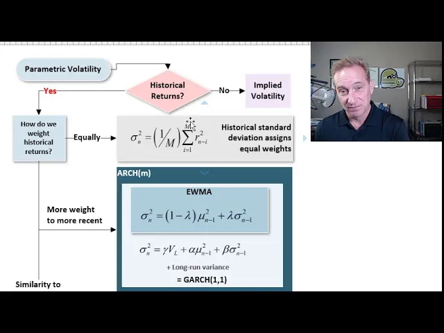
I have a diagram that tries to address that volatility as the key parameter in the parametric approach where we have lots of different a whole menu of choices but my diagram here tries to just reduce this to its essence and remember we're trying to we want to go parametric now and we want to say we want to answer the question what's our best estimate for today's volatility and that's a more profound question than it seems because here's something philosophical volatility is has no instantaneous existence unlike asset price we can look that up volatility is actually

a measure that requires a time series or some other assumptions has no instantaneous existence yet we're trying to estimate the volatility today and actually going forward so what I have here is this first sort of gating question are we using historical returns to inform our estimate of today's volatility you notice I do have a choice here we can say no let's not do that let's use implied volatility which is profoundly convenient but requires us to have two things a pricing model and here's the other thing we sometimes don't have a traded or observed price the

most common instance here application here is the implied volatility for an option right if if we have a model black Scholes option pricing model and if we have traded prices for the options then we can then we can use the traded prices which are normally outputs in the model to reverse engineer what implied volatility would solve for those observed prices and so we can retrieve an implied volatility without any data all of the information comes from the traded price super elegant and sensible but oftentimes we don't have the price okay now if we do use

historical returns you notice here I have a yes and then the key question here becomes how do we weight historical returns and the most common approach here is we weight them equally or that's when you see computations or discussions of standard deviation as volatility most often its equal and sometimes it's implicit because it's unweighted with even if it's unweighted it's implicitly equal so that formulas shown right here we're in the perhaps familiar to you formula for an estimate of today's variance I have Sigma Squared's subscript of n to denote today and oftentimes it's easier to

just deal with the variance knowing that we just take the square root to get the volatility right in this context volatility is a synonym with standard deviation so then I have here what I think is the most elegant and easiest formula for today's estimate of variance it's the historical standard deviation where all of the squared returns are getting the same weight here we have the returns they are squared it's over some historical window going back M days probably M periods really but probably M days and so this formula is so convenient that we can actually

describe it very easily in words and here I'm going to describe it in words now the estimate for today's variance is the average squared return very simple right taking the square root turns divided by M because we're making a couple of simplifications we're assuming that the average return in that series is zero and we're dividing by M instead of M minus one I've covered those technical nuances in my earlier playlist and our topic - those are quantitative topics for now this is fine as an estimator of today's variance and it is simple but it has

one glaring weakness at least we think in finance and that is all of the returns are getting the same weight so if M is 250 for 250 trading days over the past year then you'll notice yesterday's return is getting the same weight as the return one year ago and generally we don't like that generally we think yesterday's returns to have more weight so you notice I go here how do we weight the historical it turns well let's give more weight to more recent returns right that's the next step in up in sophistication and you notice

I have a box here for art one one at the fancy term for the very broad class of models here that have the flexibility of waiting this return and actually all it really does is add a little alpha weight here and lets us customize the weights applied the returns however I'm concerned with a subclass within arch M that really is GARCH 1:1 and exponentially weighted moving average here's the GARCH 1:1 after anyone studying this will become familiar with it eventually and the thing about the both of the models in this box is that they give

more weight to recent returns and in fact it's specifically an exponentially declining weight to the weights and constant proportion both weights yes that's true of GARCH as well math is not so difficult to show so the guards 1:1 we have here and then you'll notice it's expect it's a special case of the arch 1 1 then if I just take the weight assigned to the long run or in the conditional variance and that weight here happens to be denoted Greek Gama and if I give it zero weight then that cancels and the GARCH 1/1 in

general collapses to the exponentially weighted moving average and so I'm rounding off a little bit here or making some simplifications but we could say the exponentially weighted moving average is a special case of GART 1/1 or garth-1 one generalizes the expects potentially weighted moving average both share in common this this feature that more recent weights get greater return and in fact they decline exponentially and you can see here in the model the beta end GARCH 1/1 maps to lambda in the X months weighted moving average as does alpha to the 1 minus lambda term but

that's the feature of these two models this class of the arch arch m and then so what are these two have in common or what do these have in common really well the weighting of the returns a function of time more recent gets greater weight here we have no discrimination in the weighting the returns and so that's why finally here we have the third sort of approach to volatility as the key parameter and the parametric approach to var and here we have similarity to economic state and I'm just being very conceptual here here's the kernel

function but this is described in the first reading that's assigned frm candidates and here are the variance also has squared returns but now it's not a function of time rather there is a vector of key variables and perhaps these are macroeconomic variables for example the interest rate term structure or GDP growth and we have a vector of variables and we say what we described today in terms of those vectors what is the term structure look like today and then each day in the window we go back and compare the state of those variables and so

it's a comparison of vectors and we may go back to 230 days ago and find that in terms of comparing the vector of our variables 30 days ago is very different so it gets a low weight we may go back a year and find that in terms of our the variables in our vector it's very similar to today and we give it a higher weight so you see how in the kernel function it's not about time which is sort of a simple role it's more it's customized per via our kernel function to the similarity of

the past to today so that makes a lot of logical sense I think and so that's the schematic in terms of again the parametric volatility all of which gets to that single question what's the best estimate of today's volatility or if you liked today's variants and in turn in turn that parametric volatility is a parameter in our parametric approach which is just one of the three approaches to Value at Risk right these are all Value at Risk approaches okay so that's a summary overview of the introduction to topic 4 and part 1 of the frm

if you liked the video please subscribe to the channel and you'll be notified of our updates thank you