so welcome back today we're going to cover model selection and regularization but we have a special guest my former graduate student Daniella Whitton hi welcome Danielle thank you Daniella is not University of Washington but maybe you want to tell students a bit about yourself and how you got to be here yeah well I um in college I studied math and biology and when I was graduating I knew I knew at a grad school in something but didn't really decide on one particular thing that I wanted to study for the rest of my life and so
I ended up doing a PhD in statistics and I was lucky enough to do it at Stanford with Rob and I graduated in 2010 moved up to Seattle and I'm now an assistant professor at the University of Washington in the biostat department there and uh I didn't invite Danielle here just because she's she's a great student and friend but also she's a co-author of the textbook and this this course is based so uh Danielle and I are going to give today's talk together so we're going to talk about model selection regularization so let's recall the
linear model we've talked about already in the course we have response variable Y and we're going to model it as a function of some predictors or features X1 through XP and we've talked about least squares for doing that uh earlier in the course and in in later on the course we'll talk about ways of making that model more General making it non-linear for example or uh we'll we'll have um additive or not but non-linear models in chapter in the the lectures that cover chapter seven we'll consider non-linear models in chapter eight things like trees and
boosting but today actually we're going to stick to the linear model and talk about a different way of fitting the linear model why well because of the the model although it's very simple and it's actually been around since probably the 1920s and 1930s uh is a it's a very important model because it's it's simple which means it can be interpreted there's a small number of coefficients typically if we have a small number of features that are important it all it also it predicts future data quite well in a lot of cases despite the fact it's
simple so we want to talk today about ways of of a finger model that improving on least squares by selecting or shrinking the the coefficients of features to make the model more interpretable and in some cases to predict better so we'll talk about a number of methods of doing that today um and I'll just say a little more about these the two objectives when the number of features is bigger than the number of samples and we've talked about that in the core survey this is a situation that comes up more and more often these days
where we have a lot of features you measure on patients or in business maybe on a stock or um um in other situations you can it's cheap to measure things now and it's often the case when that P might be much bigger than the number of samples so in that situation of course we can't use fully squares because these the solution is not even defined so somehow we have to reduce the number of features and thus becomes more and more important not just to obtain a solution but to avoid feeding the data too hard so
when we um want to predict better well it will shrink or regularize or select features in order to improve the prediction and along the same lines that we have a small number of features the model becomes more interpretable right if we if we hand our collaborator a few hundred features and say these are important that might be hard to interpret if we compare them down to the most important five or ten it becomes a a it's easier to interpret and from a scientific point of view more useful so we call uh feature selection is is
a way of of choosing among features to find the ones that are most informative so we'll talk about three classes of techniques in today's lecture subset selection where we try to find among the P predictors the ones that that are the most related to the response and we'll see different flavors of subset selection um best subset selection we'll we'll look we'll try to look among all possible combinations of features that found that find the ones that are the most predictive and then we will talk about four and and backward stepwise methods which don't try to
find the best among all possible combinations but try to do an intelligent search through the space of models so fourth step wise backward stepwise in all subsets and then some more modern techniques known as shrinkage methods in which we don't actually select variables explicitly but rather we we put on a penalty to penalize the model for the um the number of coefficients or the size of coefficients in various ways so we'll talk about Ridge regression and the lasso in the shrinkage section now finally in the third section Dimension reduction we'll talk about ways of finding
combinations of variables extracting important combinations of variables and then using those combinations as as the um the features in regression we'll talk about PCR principal components regression and partial least squares in that those settings so three different classes of math three classes of methods we'll talk about today the things about today's lecture context of learning aggression so if you're trying to predict some quantitative response and you want to fit a less flexible but perhaps more predictive and also more interpretable model these are ways that you can shrink in a sense your your usual least Square
solution in order to get better results but these can just as well these Concepts can just as well be applied in the context of logistic regression or really your favorite model depending on the data set that you have at hand and the type of response that you're trying to predict and so so even though linear regression is really what we'll be talking about here these these really apply to logistic and other types of models okay so Danielle is going to first of all tell us about subset selection so best subset selection is a really simple
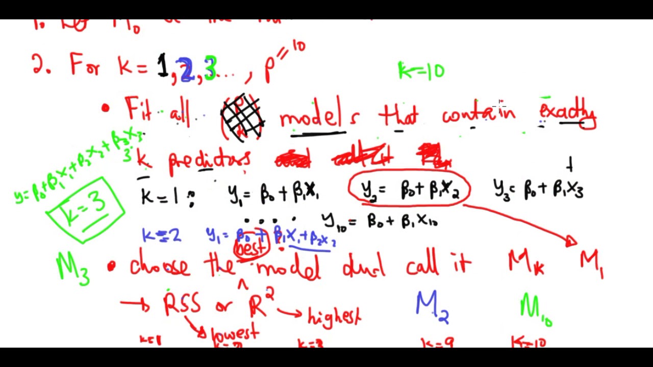
idea and the idea here is suppose that we to actually have a simpler model that involves only a subset of those P predictors well the natural way to do it is to consider every possible subset of p predictors and to to choose the best model out of all out of every single model that just contains some of the predictors and so the way that we do this is in a very organized way we first create a model that we're going to call m0 and m0 is the no mod is the null model that contains no
predictors it just contains an intercept and we're just going to predict the sample mean for each observation so that's going to give us m0 and now we're gonna we're gonna try to create a model called M1 and M1 is going to be the best model that contains exactly one predictor so in order to get M1 we need to look at all P models that contain exactly one predictor and we have to find the best among those P models next we want to find a model called M2 that's going to be the best model that contains
two predictors so how many models are there that contain two predictors if we have if we have p predictors in total and the answer is p choose 2. so if you haven't seen this notation before this is this notation is written like this it's pronounced choose so this means P choose two and it's equal to P factorial divided by 2 factorial times P minus 2 factorial and that is actually the number of possible models that I can get that contain exactly two predictors out of P predictors total and um so I can consider all P
choose two models containing two predictors I'm going to choose the best one and I'm going to call it M2 and so on I can keep on getting the best model with three predictors four predictors and so on up to the best model with p predictors so if I'm choosing the best model out of all models containing three predictors in order to get let's say M3 I can do that in a pretty straightforward way because I can just say that out of all models containing three predictors the best one is the one with the smallest residual
sum of squares or equivalently the largest r squared and so in this way I get a best model containing 0 1 2 all the way through P predictors I've called them m0 m1m2 all the way through MP and now I'm on to step three and in this final step all that I need to do is choose the best model out of m0 through MP and in order to do this actually um this this step three is a little bit subtle because we need to be very careful that we choose a model that really has the
smallest test error rather than the model that has the smallest training error and so there are a number of techniques that we can use to choose a single best model from among m0 to MP um NDS include prediction error estimated through cross-validation um as well as some methods that we're going to talk about later in this lecture which you might not have seen before and these include mallow CP Bayesian information Criterion and adjusted r squared so we'll come back to some of those topics in a few minutes so here's an example on the credit data
set and we saw this this data set in one of the earlier chapters and this is a data set that contains 10 predictors involving things like number of credit cards and credit rating and credit limit and the goal is to predict a quantitative response which is credit card balance and so what we can do is um we can look at every single model that contains a subset of these 10 predictors and these models are actually plotted here on the left hand side so here this x-axis is the number of predictors it actually goes from 1
to 11 because one of these predictors is categorical with three levels and so um we used a couple of Demi variables to encode that and on the y-axis is the residual sum of squares for each of the possible models so for instance like this dot right here indicates a model that contains one predictor with a pretty terrible residual sum of squares and all the way down here we've got a model with 11 predictors that has a pretty decent residual sum of squares so the reason that there's a lot of dots in this picture is because
there's a lot of possible sub models given 10 total predictors and in fact as we're going to see in a couple minutes there's 2 to the 10 sub models so there's actually two to the 10 dots in this picture although some of them are sort of on top of each other and so this red line here indicates the best model of each size so this red this red dot right here is m0 that's excuse me it's this is M1 what I just what I just showed you is M1 so that's the best model containing one
predictor because that is the smallest residual sum of squares this is the best model containing two predictors this is M3 best model containing three predictors and so on so when we perform best subset selection what we really do is we Trace out this curve to when we get m0 through MP and now we're just going to need to find a way to choose you know is M10 better than or worse than M4 and so on we're just going to have to choose among that lower Frontier so so on the left hand side here we see
a number of predictors against residual sum of squares and on the right hand side we've got number of predictors against r squared and as we saw in chapter 3 r squared just tells you the proportion of variance explained by a linear regression model by a least squares model and so once again we see a whole lot of gray dots indicating every possible model containing a subset of these 10 predictors and then the the the red line shows the best model of each size so again this is the M1 that we saw earlier this is M2
over here is M10 and um what we notice is that as the models get bigger as we look at larger and larger models the residual sum of squares decreases and the r squared increases so um do we have any idea of why that's happening maybe Rob can tell us I can tell you yeah so it's because as you add in variable things cannot get worse right if you have a subset of size three for example and you look for the best subset of size four at the very worst you could set the coefficient for the
fourth variable to be zero and you do the same as you'll have the same uh error as for the three variable model so the curve can never it can never get worse it can be flat if you clear the slide here we can see it looks like it's actually flat from about three predictors onto from three above up to 11. but it's certainly it's not going to go up but it can it can it cannot it can go be flat as it is in this case but we can't do any worse by adding a predictor
and actually what Rob just said relates to the idea that um you know remember on the on the previous slide here in step three when we were talking about best subset selection we had this step and I said that in order to choose among the best model of each size we're going to need to be really careful we're going to have to use cross validation or CP Bic adjusted r squared and that really relates to what's going on here because you know if if I ask to you hey what's the best model with eight predictors
you'd say okay here are all of the model with models with a predictors and like clearly this is the best one it's got the smallest residual sum of squares there's no argument but if I ask you which is better this model here or this model there Suddenly It's Not So straightforward because you're kind of comparing apples and oranges you're comparing a model with four predictors to a model with eight predictors you can't just look at which one has a smaller residual sum of squares because you would because of course the one with eight predictors is
going to have a smaller residual sum of squares so in order to really in a meaningful way choose among a set of models with different predictors we're going to have to be careful and we'll talk about that in a few minutes good