we uh learned about model selection and uh complexity control in general we also learned about uh radial basis function in neural network and uh I'm going to make what we have learned about uh complexity control more Concrete in terms of mathematics behind uh this notion and then we will see how this can be more precisely applied to to uh radial basis function complexity control model selection as well as uh neural network okay so so I'm going to uh talk about model selection today or complexity control so selection or complexity control uh recall that you know
I told you that usually we have an underlying function f but we do estimate a function given data which we call F hat and we would like our estimate to be close to the true function but there's always a relation between bias and variance you know bias squar plus variance would be minus square error okay so that's what we would like to minimize but depends on the complexity of the model we are either minimizing we are either decreasing the bias but increasing the variance or vice versa you know we Fe align to our data say
for example in regression it's high bias but low variance but we feed a polinomial of degree n minus one to n data it's very high variance but it's low bias right and we need to have a basically a tra a tradeoff between these two and find minimum minus Square okay I'm going to define t to be a set of data say I have n data point this is my training set I assume that each data point Yi is f of x i when f is true underlying function plus some noise okay so this F is
true function and Epsilon is some noise so we are assuming that it's Gan noise centered at zero with a standard deviation Sigma okay so I assume that the noise is additive noise in terms of notation uh now F hat will be my estimated function and F hat of x i I call it y hat okay also uh you know for Simplicity sometimes I use fi and I mean f of x i and I would say F hat I and I mean f hat of XR okay so usually you know we have this training set we
feed a function to our data and this function gives us some y hat right and we are minimizing an objective function when this objective function is basically summation over y i and y i hats right this is usually what we minimize as our objective function you know this our empirical error and we had this discussion in the previous lectures that this empirical error you know always decrease but true error decrease up to some point and then it start to increase and the optimal model would be a model which has minimum error on the uh I
mean minimum true error not minimum empirical error that's our empirical error and minimum true error is different from this okay okay so uh in in uh practice that's the objective that we're usually Trying to minimize which is biased downward you know it's not a good would estimate usually of the true error it's bias downward and we would like to take care of this bias somehow okay uh you know given given this point if I write this quantity expectation of uh y hat minus y this is you know Y is my observation y hat is when
I Feit a function to the data and I estimate some you know I have some prediction and in in the process of minimizing the empirical error that's you know one of the term that I'm minimizing if I look at the expectation of the term time minimizing in empirical error let's more closely look at this term and see what this term that we are minimizing is and what does it mean you know this is a y hat that I estimated from data and Y and Y is uh f plus Epsilon right there's a true function that
has been distorted by Some Noise Okay that's that's my observation y so my observation Y is basically F the true function minus Epsilon the noise okay so I will write it as y hat minus F minus Epsilon squar so I just group these two in one group minus epon and now it's a squar so it is y hat - F SAR plus Epsilon squar - 2 Epsilon y hat minus F okay okay now this is expectation of uh y hat minus f s plus expectation of Epsilon squ minus 2 expectation of Epsilon y hat minus
F okay this is my estimation this y hat is my estimation so y hat is basically F hat you know it doesn't matter if I I mean it's just let me just write it f hat so that's my estimation that's the true one this is basically what I need to minimize see what I need to minimize is the distance between true function and estimated function but an empirical error what I minimize has other terms as well I'm minimizing the true error plus two other terms so if I really would like like to uh minimize the
true error I have to take care of these two terms somehow so I don't have access to f f is unknown right I do have access to this quantity so left hand side of this quantity is noun if I can estimate these two quantities then I do have an estimate of the true error so so let's see if we can estimate these two terms so expectation of Epsilon squared what is it it's just Sigma squared right because Epsilon was normal distrib has normal distribution centered at zero and the standard deviation was s okay what about
this term is it zero why it's zero fixed with respect to X is given so why Y and they are fixed they're just constant so that that term is the expectation of so it's thean it might be more clear you know this is why hat if I tell you that this is f hat you know this is my estimation if I change Epsilon F will not change right f is true function what about F hat if I change the noise of the data does it change my estimate or it doesn't no you know I give
you this data and tell you to predict a line for me I add the noise now predict a line for me it doesn't change your estimate it does change your estimate if I change the noise of the data I have a new setup observation and I do estimate my function using my observation so changing the noise will change my observation will change my estimate okay so I can't say that this term is zero in general in some cases it has but not always let's let's consider you know different cases more carefully so case one in
case one I assume that the this data is not in the training set okay so I just I was looking at empirical error of a given data point point and this sta Point suppose that is not in the trainings if this sta point is not in the training set that you're are right that this term is zero you know because I estimate my function using my training set and I have an estimate F hat here I'm talking about y0 or Y y null which is not a part of this it doesn't matter how much I
change this y it doesn't matter how much I change the noise of this y it's not even a part of end points that I use to train my model you know it has nothing to do with the model that I estimate so this cross term will be zero if my Observer if this y null is not a part of the training cell okay so uh this cross term in this case will be zero to see it more I mean clearly can say that this Epsilon is basically in fact um you know this Epsilon is Yus
f so it is y minus F and this is f hat minus F and this Yi is not in the training set and F is constant you know is true model and this is an estimate which has nothing to do with this y because y hat is not in the training set so this is going to be zero it's like covariant of Y and F hat and these are independent now y had I mean f is independent from y so this is going to be zero in this case okay so it's going to be zero
in this case so any questions so far is it clear okay so um so since it's zero I can say that expectation of um this expectation squared is equal to expectation of F hat minus f s plus Sigma squ and the third term is zero now that was for one point if I sum Over N points but this m points are not a part of training set I just choose M points that are not in the training set if I sum over M points that are not in the training set then basically I have summation
of all y i hat minus y i squar i = 1 1 to m is equal to summation of f i hat minus fi squared plus summation of Sigma squ okay so the summation of Sigma squ I mean Sigma is constant so it's it's just m Sig squ okay this is the error that I was looking for the distance between true function and estimated function let me show it by this notation and this is my empirical error the error that I can basically is distance between my observation and my estimation but in this case I
I choose points that are not part of the training set I have already trained my model then I introduce points that are that that that are not in training set and my model has some prediction for that and I'm looking at the distance between prediction and Y okay so let me call this I mean show it with this notation so here we had our notations let me add these two this is my true error and this is my empiric color so this basically tell me that true error is empirical error minus M Sigma squ which
is a constant okay so in other words empirical error is a good estimate of the true error up to a constant in this case so in this case for it means that I would like to really I would like to minimize the true error but suppose that I minimize in prolor that's okay because it's an estimate of the true up to constant so if I minimize this it's as if I minimize this because this constant has nothing to do in I mean has no effect in my optimization I'm trying to find a model with Optimum
complexity so if I go go for Optimum complexity that minimize this quantity I can assure you that it has been minimized this quantity as well this is the main justification behind cross validation in Cross validation we are training a model using training set but uh when we want to decide about the complexity of the model we are checking this with a validation set do you remember you know we had that was our training set where we took a part of data we set it aside call it validation set okay and this is the training set
and we are learning the model using this but we are testing the model using validation set a data that model hasn't seen so far and we are trying to minimize the error here so when you're when you're minimizing the error here your estimation your empirical error is a good estimate of the true error so if you Min if you have a model which minimize your validation error then you have minimized the trer okay so so this is this is the main uh justification for CR validation so the more interesting case would be the case that
this data is in the training set so quite often we we are minimizing training error and that's where overfitting happens right because it goes down all the way when you add the complexity so let's see what's happening in this case so in the case that this data is a part of training set so when this is a part of training set you know everything goes fine except that this cross term is not zero anymore right so basically our question is that can we estimate this cruster okay so can we estimate this any idea yes this
so basically you're assuming that there's a close form for Fad in terms of Epsilon but it's not the case in most of the um most of the time right and most of time you don't have close form estimate for fat you have a neural network and the output is just some f hat you can't write it in a Clos form even in the cases that you can write it in closed form it's not in terms of EP epon you know I fit a polom it's not in terms of Epsilon so uh this estimation is not
trivial okay uh we have to use Stein's Lema to to estimate this so what is a Stein's LMA basically it says that if there is a random variable X let me write it here if there is X which has normal distribution Theta Sigma squ and suppose there's a function G and and this G is differentiable function you can take um derivative of this function so it's enough if it's vly in differential so if you have this then expectation of x - Theta GX according to Stein's LMA is just Sigma squar expectation of derivative of G
with respect to X okay so X is normal this has normal normally distributed x minus the mean of X time G and G is an arbitrary function but the condition is that you can take derivative of G if you want to compute this expectation expectation of product of these two terms when one term is normal distribution and the other one is a function of this random variable then this expectation is Sigma squar when Sigma was standard deviation of this normal and expectation of derivative of this G with respect to X okay okay let's apply this
Stein's LMA to our problem our problem is to estimate this uh basically cross ter here so how can I apply Stein's LMA here tell me what would be if I just want to apply this LMA here what would be my G what would be my X sorry okay is Epsilon right so basically you know this is my Epsilon because Epsilon was normally distributed centered at zero so so this is basically Epsilon minus 0 right and then G is this term because fat is a function of Epsilon right so F hat minus f is this G
so this is my G and this is my x - th see I mean fat is a function of this f f is not a function of Epsilon but fat is so fat minus f f is a function of Epsilon Okay so so according to Stein's LMA this is going to be Sigma squar expectation of G derivative of G which is f hat minus f with respect to x with respect to Epsilon so this is Sigma squar expectation of derivative of f hat with respect to Epsilon minus derivative of f with respect to Epsilon so
what's derivative of f with respect to Epsilon it's zero because f is independent from Epsilon right so no matter what your noise is it doesn't change your underlying function underlying function was a function prior to your observation right observation was the true function Disturbed so it doesn't matter how much you disturb it you know the true function was true function so they're independent this is zero so this is Sigma squared EP expectation of derivative of f hat with respect to Epsilon so I can go one step further I just write a chain rule here this
is f hat I I would say with respect to Y my observation times y with respect to Epsilon okay what's the second term derivative of y with respect to Epsilon just remember that y was F + Epsilon now derivative of y with respect to Epsilon is derivative of f with respect to Epsilon which is zero dtive of Epsilon with respect to Epsilon is one right so derivative of y with respect to Epsilon is one which makes sense because derivative means I I perur this variable how much this variable is going to change so Y is
f which is a constant plus Epsilon I perb Epsilon I change my noise how much my my variable how much my observation is going to change exactly the same you know because it's constant plus the noise so you change the noise exactly the same your observation will change so I can write my cross term as Sigma squar expectation of derivative of my uh estimation with respect to Observation this is an interesting term in terms of concept derivative of my OB dtive of my estimation with with respect to Observation you know suppose that this is my
observation and my estimation is just a linear function this is my f hat so this ST means I perur one point you know I change one of this point how much my estimation will going to change okay consider this case when my estimation is a linear function with this case you know I have the set of same set of points but my estimation is not a linear function it's quite a complex function it goes through all of this point if I preter one point only you know I have to see how much my estimation will
change due to this per I do the same thing here I change this point to this point do you think this quantity is going to be larger here or larger here larger for the complex one right so in in this case that my function is a complex function if I perur a point my estimation will change a lot when it's not a complex one it's low complex function when I perer a point my estimation doesn't change much so we can think of this as a measure of complexity of the model model that you are fitting
okay so we let's call this D so D is just this derivative derivative of estimation with respect to Observation a particular point okay now yes does that also mean that as you have more sample points your like if you have more uh samples the degree to which each one influences your final small so does that mean we get closer to the actual if you have more data your estimation your final estimation it means will be more robust right but I'm talking about a I mean our estim I mean Point estimate my estimation at a single
point right so that yeah I mean if I write the summation over all of these points basically I need to compute the summation over all points of this quantity right how much if I perer each of these points separately in total how much my model will change so it's independent of the sample size that that rate change it is not independent of the sample size but I think you can directly conclude that if your sample size is large you know this quantity is going to be a small right okay but it's not independent so in
this case uh you know that was remember you know that was the quantity that originally we start to work with so we have this term this is true I mean this correspond to True error we have this term and we didn't know how to calculate this cross term and now we know what this estimation is so basically uh this is going to be this term plus Sigma squar - 2 Sigma squar this quantity now let's sum Over All Points say end points but in this case all of these end points comes from training set so
we sum over all end points uh there these points are from the training set so summation Over All Points here actually would be sum I = 1 to n of y i hat minus y i² is equal to sum over all points of f hat minus f squ plus summation I = 1 to n of Sigma s which is n Sigma s minus 2 Sigma squ summation of di where Di is just Sigma of fi hat with respect to Yi so this is a measure of complexity okay let me just use the notation that I
used before so this is my empirical error this is my true error this is a constant this is not a constant anymore this is a function of the complexity of the model so when it was not a part of training set I didn't have this term so minimizing this was the same as minimizing this because that was constant with respect to the complexity of the mod now I have a term which is not a constant with respect to the complexity of the mod so this goes up when the complexity goes up right so the true
error is imp prol error minus a constant plus 2 Sigma s a function of complexity this is called Ste unbiased risk estimator in short they call it sure Stein's on biasc estimate so it is times unbias risk estimat so it is sure so can we estimate the cross term sure uh okay so see when uh you know it it gives you now a very good uh Insight that why we have this Behavior you know empirical error when empirical error is training error you know when we are using the the data points that we have seen
in the training set goes down all the way when you add the complexity of the model so this is always decreasing this is constant I even don't care about it in terms of minimization but this goes up when complexity goes up with low complexity it's small with high complexity it's large so I have this function plus a function which has completely the opposite Behavior it's a small here it's large here so this this part has a behavior like this and together you know together they have this Behavior you know this is what we observe about
the true error you know that up to certain model it goes down and then it start to go up it start to goes up because of this quantity because there is a there's a function of complexity which will be which which is going to contribute to the true error okay and that's why we observe this any question yes so the empirical error could be larger than the true error when the when a model is not very complex the true error the empirical error could be larger than the no because you have this constant as well
you know it's always biased downward you know in when when model is not complex it's pretty small and you have empirical error minus you know some value would be the true error yeah the true I mean you're saying the empirical could be larger yes yes okay so it is interesting theoretically but it uh gives us some indication or some you know Direction how to go for complexity control and find the optimum number of optimum complexity in some case so in particular I'm going to show you how can we use Shure orin's unbias risk estimator to
find the optimum complexity of radial basis functions okay so let's get back to RBF radial basis function and see how can we compute the optimum complex so recall that uh the complexity of RBF is controlled by the number of radial bases right so the more nodes that we have the more complex the model is the less note that we have the less complex the model is it's we had this uh discussion in the previous lecture that you know this nodes can be roughly uh interpreted as mixture of different Gan you know as you have more
Gan you're modeling your data with more Gan compared to less number of Gan for example but in general you know it it contributes the complex ter so uh we had you know uh W in terms of fi and we had if you just remember remind me what was this values that we computed in the past you know we had this is input X1 to XD then we had m f that was 51 that was 5 m and we had some output you know and if you remember we defined X to be like d byn of
our data and then f was M by n and then we had Y which was like uh K by n and we had W which was M by K then we computed W in terms of by minimizing you know by minimizing Yus W transpose 5 using list Square we computed W what was that W five five transpose inverse five y transpose okay so that was five transpose that was five okay so that's our W right if this is my w my w hat sorry my V hat is going to be W transpose Time 5 right
so my estimation in this model is W transpose Time 5 which is um y f transpose five F transpose inverse transpose * 5 so to get rid of this inverse transpose let me transpose both s side of this equation so y hat transpose is uh F transpose five F transpose inverse f y transpose okay that's my estimation you know that's F this is my observation what radial basis function does is to estimate uh the function using this equation and this equation you can see that it's linear you know this is a linear transformation on y
so it give me y I apply a linear transformation on Y and I give you y hat okay because five is just constant right so I I decide about the number of nodes I decide number of nodes to be two to be three to be 10 I decide about number of nodes and then I compute this five for every uh data point and put it in this n byn Matrix then I compute five transpose five F transpose inverse 5 this is a transformation now I apply this transformation to my y to my observation let me
call this transformation h for so why hat is H * y when H is just constant here right okay um you know why hat we have K outputs for Simplicity let me assume that I have only one out output then you can see that if you want to extend it to K output that would be uh trivial to extend so let's assume that the number of output nodes K is is equal to one so I have only one output note so in this case this y hat which was K by n is going to be
1 by n and I had sorry a transpose here so and the why had transpose would be n by one right so it is a vector now I just write it this way so y transpose is H uh Y is it clear I just assume that we have one single output so this Matrix is which was K by n originally now it's 1 by n n 1 by n is not a matrix it's just a vector I just change my notation you know you can still keep your notation just I thought it's more convenient to
or more clear to explicitly show that it's a vector it's not a matrix okay so suppose that I want to apply sh Stein's unbias risk estimator I want to estimate the true error of RBF the true error would be empirical error minus n Sigma s + 2 Sigma 2 6 sum over di when di is just derivative of fi with respect to Yi this is my fi hat this is my estimation so if I want to apply sure to RBF I have to take derivative of my estimation with respect to one data point okay so
this is why hat or this is my estimation so I would like to apply sure to RBF and um I need to compute di which is derivative of fi hat with respect to Yi so what would be what is fi hat in RBF you know this is n by one vector which is estimation of all of my end data point for data point number X for data point I with index I for x i or for observation Yi what would be my estimate you know I have this n by1 Vector which is just H times
y y is n by 1 and this H should be n by n you know this H should be n by n f is M by n f transpose is n by m m by n and this is five I transpose M by m so H is n by n okay so I have this n by n Matrix H * n by1 Vector y it gives me n by1 estimation by hat so what would be fi means what would be this particular s sorry the I's row of I times Yi right sorry you are talking
about the derivative yeah okay so so basically fi hat which is show it by y i hat as well would be this row means row number I of H so I show it with this notation it's like math lab notation you know row I all columns times y it's vector and this is scale now I need to compute di which is derivative of this fi hat with respect to Yi basically I need to compute derivative of h i all columns times y with respect to Yi with respect one of the elements of this Vector what
this uh derivative is going to be let me write it this way you know the h i * y means this row times this column right it is basically H i1 * y1 you know this element times this element this element times this element plus h I2 * Y 2 plus h i i * y i plus h i i + 1 * y i + 2 plus h i the last one n * YN I would like to take derivative of this with respect to Yi it's going to be hi I I right so
everything will be zero except you know they're not dependent on hi except this one so when you make this multiplication you know no one has any effect except that the corresponding uh element on this row of H so this is hii I mean di is hi II so let me write sure for uh this case the true error is empirical error - n Sigma S Plus plus 2 Sigma s summation over I to n of hi I I okay what is summation over I mean summation from I to n of hi I I it's trace
of H right so true error is empirical error - n Sigma s + 2 Sigma squ trace of H okay now let's see if we can know what the trace of H is Trace of H is Trace of five ter ose five F transpose inverse five and F is a constant that we computed here right so I can compute this Trace so this is equal to trace of you know I can take this F here right trace of five F transpose times 55 transpose inverse so 55 transpose * 5 Pi transpose inverse is identity so
it's trace of identity what the size of this identity you know this F is M by n and this n by m and it's also M by m so it's ident I mean the size of this identity is m M so what's the trace of identity with size m is m m was the number of nodes that we had right and conceptually we knew that this quantity has something to do with the complexity the more complex model have larger quantity di now we realize realiz that it is in fact this summation is in fact the
number of nodes which is the complexity of our RBF you know the the larger the number of nodes are the more complex the model so basically in RBF the true error is empirical error minus n Sigma squ plus 2 Sigma squ * m so you want to choose the right complexity you have to minimize the true error not in precolor but to minimize the true error you can simply start with m equal to 1 compute this quantity then m is equal to two compute this quantity and so on at some point you know you see
that this true error is start to increase you know it comes down down down it start to goes up with some M that would be the optimum M you shouldn't go further than that you know it should have stopped there so basically you can find the optimum model for rvf any question here yes no you don't need to do cross validation because you can estimate the true error correctly just using your training St okay so what about Sigma you know Sigma we assume has normal distribution has been added to uh the true function and it
generates the observation now I have to compute the true error and this true error has to do with the standard deviation of this noise but what I have been given is just some observation you know just give me this XY so what would be my Sigma so we don't have this Sigma we have to uh estimate it right so I have some observation and I have some estimation and over my data point I can compute the you know standard deviation or compute the variance but the thing is that if if I replace this Sigma here
with this quantity you know this y Hat by itself is a function of complexity you know the more complex the less um the the smaller this value and the smaller this value so in PR practice in cases that we have this situation we don't consider this why had to be a function of complexity we usually estimate the sigma with a low uh with high bias and low variance estimation say for example a line so simply fit a line to the data use the Y hat of this linear function compute the sigma and consider the sigma
constant over the estimation don't change it you know when you change the complexity of your model don't change it so really you know Sigma doesn't change with the complexity of the model and we need to estimated at some you know some way we need to estimate the true estimation would be you know according to the true model but we don't know what the true model is let's assume that you know a very High bias and low variance is the our estimation at the beginning you know set it there and then don't change this is usually
what we do in practice okay any question so uh uh if you look at uh sure you know sure was true error is um imperical error minus constant + 2 Sigma s this quantity and we learned that this quantity is a function of complexity right so if I want to minimize error with respect to the complexity instead I can minimize imp pral error this is constant + 2 Sigma s d i this is function of complexity this is justification behind regularization you know one way of complex control which is very popular way is regularization regularization
means that in of minimizing your training uh your objective function add a penalty to your objective function and this penalty is a function of your complexity it goes up where your complexity goes up okay so regularization means that you have a function which you usually minimize that's your objective function add a penalty to this function which is a function of complexity so in this case you know be Computing this derivative is hard it was easy for RBF in general it's not easy so let's all together forget about estimating this derivative but we just know that
this derivative is a function of complexity which has this form and is going to be added to this form and produce a function of this form so let's just add a function which increase by complexity and there are other different type of penalty function that you can add here would be L2 Norm L1 Norm L2 plus L1 Norm all type of regular okay in in all sort of model selection it's called regularization and we're going to see some particular C and one particular case of that which is weight Decay for neural network in next lecture