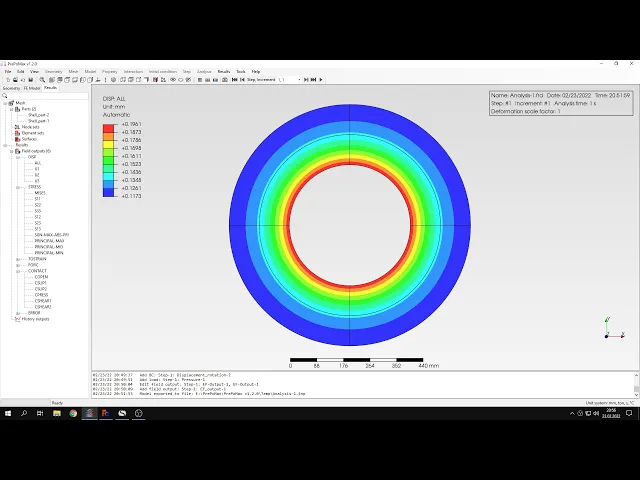
hello and welcome to my next tutorial about prepomex this time i would like to show you how to perform a plain strain analysis of a composite pipe so let's create a new model first i will choose the plane strain analysis and defaulting system and i will import the importer geometry now and this will be the composite pipe geometry as you can see it's a surface again uh it was modeled in xy plane uh and the rest is is pretty much not so important in this case there are some special considerations for axis metric analysis but
we will proceed to that in next video so let's create a mesh now i will use meshing size of four millimeters this will be maximum element size and i can create a mesh for both parts at the same time as you can see the measure is already created so i can proceed to the actual analysis setup let's define materials first um i will use two materials because as i said this is a composite pipe so this will be steel material and i will specify standard density for steel and the one that we pretty much always
use in our analysis and i will specify a new material this will be copper and i will define its values like this and also poisson's ratio so that's it when it comes to material properties now i have to create sections i will name this first section still and this will be applied to the outer layer of the pipe and i will specify thickness this is mainly for visualization and i will also specify properties of another section this will be named copper and the same thickness and i will apply this to the inner region of the
pipe so now we have materials and sections defined and i can proceed to contact definition because we have a contact condition between those two layers and we are interested in the pressure between the layers so we need to contact interaction this can be a tie constraint so i'll create a surface interaction and this will be service behavior heart default type and i will search for contact pairs using the new tool to detect automatically uh contact pairs so let's search for them and detect that two pairs the first one is surface with surface so we don't
need this one we are interested in edge to edge contact so i will accept this one and i deleted the previous one and now we have the the first part of the analysis prepared and i can proceed to step setup so i will define a new static step and i have to define boundary conditions of course i will use symmetry boundary condition for these two edges this will be in x direction and i will define another boundary condition for these two edges and this will be in the y direction and that's it when it comes
to boundary conditions and now i just have to specify pressure uh i'll define pressure acting on this internal edge and this will be 17 megapascals for this pressure all right so now almost everything is prepared i just have to look into the outputs i will change this output to 3d this is something we also did in previous tutorial and i will request contact output because we are interested in contact pressure but before i will submit the analysis i would like to show you something else because you may encounter some issues with two-dimensional geometry imported to
people max especially if you prepare it in frequent for example um i always prepare my geometry for permits using freecad and there are some tricks that may have to be used to make sure that normals of the faces are in pointing the in the correct direction uh it can be done in freecad there's an option to reverse the the shape i showed you this in the previous tutorial but it can also be done in prepondex i will show you this soon but i would like to also tell you that there are several ways to prepare
two-dimensional geometry either from sketch or from a 3d model in freecad one of them is something that i could also tell you you can select the sketch and use the make face from wires option to create face directly from from the sketch this is a really convenient option and then i just divided this face into two separate regions using boolean fragments and the additional sketch and then exported it to people max and if you encounter some issues with with normals as i mentioned you can go to geometry and check the normals using this option uh
flip face normal and you can make sure that the faces have proper normals here a front face should be facing our direction in this case it's correct otherwise we could select the faces and reverse the normals so it's not a problem you can do it in prepare max as well all right so the analysis is prepared and i can submit the simulation let's run the analysis now we already have the results so let's check them and now as always we will compare the results to analytical solution let's start from the contact pressure and this is
cprs variable and as you can see the output is in three dimensions because we requested this and i can hide let's say i will hide this this part of the pipe and i will check the value of c press that we expect from the analytical solution here's the the analytically calculated value and as you can see it's in very good agreement with with what we got from the simulation all right so let's bring back the visibility of both parts and let's look at them from this direction i could also disable display of mesh it's up
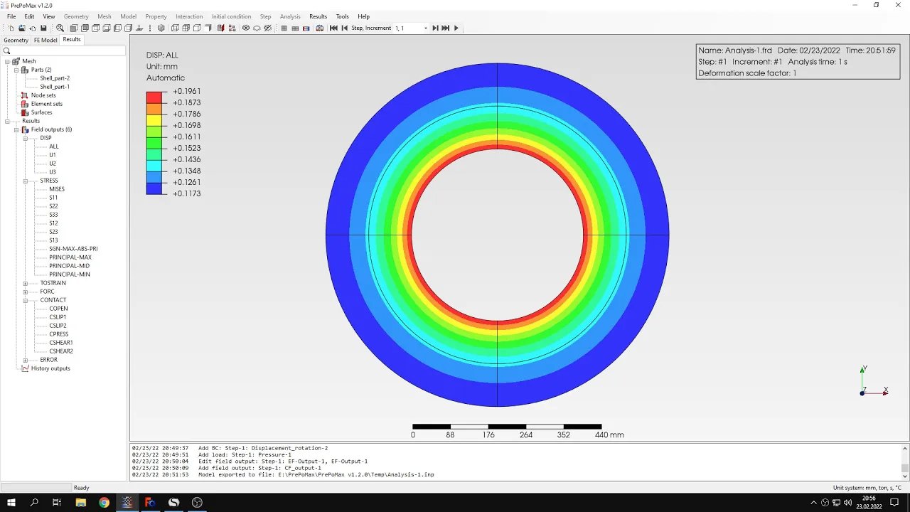
to you and now i'll switch to stresses and i will use the phone message stress and to check the develop the consistency with analytical results so for this purpose let's maybe hide one of these pipes one of these layers actually so i will hide this one and i will this the legend will now adjust to show only this inner values on this inner layer so let's compare them with analytical solution as you can see here are the results the the sheet for calculation is quite complex here but i will show you the most important parts
here i change the radius for which their stresses are computed so now they are computed for a and this is the inner radius of the inner edge and let's compare this with what we get from the simulation uh as you can see the agreement you don't even have to use the query tool as you can see the agreement is very good so now let's try let's check the the other edge this one here or the other surface actually and let's check how it looks like in analytical solutions so i will substitute this i will specify
that that the radius should be equal to b and as you can see the value now changed and here's what we get in the simulation again it's very close to the identical solution so let's now invert the visibility of of parts i don't have to do this manually i can use the predefined option in view menu to infer the visibility of display parts and now let's proceed to results for outer layer and this one is from b to c let's start from radius equal to b so and this place here and let's see how it
looks like in the simulation uh as you can see it's still very close to analytical solution and now let's check the uh value for uh final radius this will be c and let's let's take a look at the analytical solution um at the this outer radius of the whole pipe so let's see how it looks like here and now the the difference between the electrical solution and numerical one may be a bit larger but it's still good agreement and especially if you look at previous locations we can say that the discrepancy is really small and
the results that we obtained from the simulation are very good i can display both parts of the pipe again of course i could also use the uh processing transformations here and i could create symmetry vo here so you could see the uh the whole pipe in 3d not just the symmetrical parts not just the quarter of it so here's how it looks like if we display the the whole pipe we can even hide the edges so it looks like we analyzed the whole uh the whole part not just two-dimensional region and quarter of it so
that's basically it for this tutorial thank you very much for your attention as always feel free to ask any questions and suggest topics for future tutorials in the comments have a nice day and see you in the next video