Dear friends, a quick uh presentation of the central problem uh we face you know with uh statistical inference with science a lot of things in real life that's called the laws of numbers. How many observations do you need before you can be comfortable that you've seen the thing and you can make a statement with thin tail variables look um on the left here we're looking at sum of observations by n so n becomes average look what happens to your average and here when you appear on the right I don't think anything can move the average uh the distribution tends to deliver mild u tail uh you know events so it you really have uh so no big shock will have a big impact anymore. Look on the other hand at fat tail variables.

The average you keep adding information but the average keeps jumping and of course this is in norm L1 the average you could do for any norm. uh and and of course things will get worse in higher numbers. My my research on this I'm I I'm writing in parallel a book called solid risk that has comprehensive work and then there's something called incremental science.

Incremental science you take a simple point and you publish it not to lose you know sight of the big picture um I make sure that they're synchronized and and they're working together. So if I have to prove a point I want it you know put under scrutiny and put it in a journal I put it here on the left. So I'm I'm going to cover a paper with chili law on underestimation of violence using common methods linked of course to law of numbers a paper with Rafael Dadi in physica we published something on genie I'm writing a very short letter and of course a big paper on uh on central limit and and the problems you know central limit is the next step after uh the laws and of course the drafts of other papers connected to small little points because I've been working on statistical inference on the fat tails.

Now let's look at this tableau of fat tails. You what you have here in in in this yellow color is uh what really u works and in other words the place where the law of large number works. Um the general distribution means there's no randomness and of course you don't get information from a signal information bi is you know you have 0 1 - one one this kind of variation we just have two states tailed from convergence to Gaussian Gaussian and there's something called sub exponential the cut point here for those of you who do finance uh very familiar with the log normal distribution it's exact cut point uh right here so beyond that we leave the yellow area where the law of large number the weak law of large number doesn't matter strong works beautifully to what we call convergence issues you're entering something uh that has a second moment here this is category power law which we'll define and then you have something that doesn't have a second moment we call it the levy stable basin and then here there is this big important notion forget about it um that uh with alpha less than one meaning uh the distribution doesn't have any uh mean.

So you're going to be fooled because in sample you will always see me. So let let me define that class the the paret and tail again that class that is in white we call it paret and tail that you know it's formally defined as a variable that has that kind of xus alpha asmtoic behavior and of course there's what we call here slowly moving function so it can have something in the body and then when you go to the tail it becomes tail so I'm not going to define fat tails here I'm talking about statistical inference on the fat tail The simplest form of power laws what we call power law here. This is you know really I'm talking about the final power law are on on the left the easiest one to work with is parareto one.

I don't know if it has one or two parameters because it has a minimum value and alpha exponent. So the minimum value I don't know if you need to calibrate it if you call it calibration if it counts or not. It cost you nothing really.

Just take the lowest value and then or you can set your value and only sample uh what happens above. three parameters in red is because that's what I use the most where you have a scale uh you have a location the mean for a Gaussian but but this is no longer I mean we're still in a location scale something called family of distribution where you stay in a distribution if you divide x by by s or if you take minus uh m from from x so you move the distribution left or right but but um for some uh but uh but we definitely stay in a scale family of distribution but uh we have uh something that that that that is different from the Gaussian that the S here is no longer the standard deviation in in the Gaussian if I divide X by S uh you know and and of course uh S is normalized and divide by S will be a standard deviation so we map the standard deviation which is the square root of the expectation of x² or x - m square. So the now four parameters the the the beta prime uh you know you can work with it uh I'd like to work with it but this is not that important because the additional parameter they have four parameters additional par may not be worth the cost again when you go into the tail doesn't matter at all.

The two-tailed the student t is a nice way for people in finance to model prices, but you can use a double par. It doesn't make a difference because again the lower the alpha exponent and of course the more fat tailed the lower the alpha exponent. The lower the alpha exponent the more the tail matter and the body basically provides no information.

So you can have anything in the body double paro it doesn't matter it's it's the the tail that matter. And then here the levies table will work with it. Levy stable is is quite important because you can reverse to it under summation and and we can do some analytics on levy table and you don't need you know to worry about preassytoics when you work with it because again I mean the levy stable has of course the same tail alpha so this is not going to be now sample equivalents I was writing silent risk and I asked myself a We can go back to the first graph uh that we saw.

I ask myself a question. Uh on the left of course is a Gaussian on the right is some power law. Did anybody make an equivalence of how much more data do you need for power law?

It turned out that this has not been done. Why it hasn't been done? Um it hasn't been done.

Um I don't know why. Maybe because statistician aren't uh interested in power laws. Power laws usually are the domain of physicists and physicists don't really care about statistical inference.

They they're they're really spoiled by nature being very clean and very neat and uh so so they you know and and we have a lot of samples in nature. So the the the problem of sample equivalence never really came up and it's not very hard to compute. So here I'm looking for um np index by p the power law which is ng gaussian.

you set a number and looking for a equivalence okay or table of equivalents trust uh u for intuition and to realize how many mistakes people make um something I refer often in my book a pinker mistake why do I select pinker my papers I don't mention too much simply because uh he it represents this techniques represents the journalistic approach to saying oh this is my average this is evidence the sample is too stochastic for it to mean anything um So uh we we we if I take any of the distribution that we saw here and sum them up we're going to go to that basin of attraction. If the alpha is below two definitely you'll go to a basin of attraction uh the the stable distribution so I can do some analytics and I can do derivation and I can find that uh tail equivalence between the two which I did here uh and quite a shock. The shock was as follows.

When I was writing silent risk, I asked myself a question. I said I people for some weird reason select 30 N of 30 in a Gaussian as sufficient to uh gloiate about something. So I told myself, hey, you know, what if the data is parto and the one that people discuss the most is a parto 8020 meaning alpha of 1.

16. How much more data? I said maybe uh 400 but then maybe I'm exaggerating 400.

So I asked around people told me oh at least 200 or someone ventured to say a thousand. Uh yesterday when I gave the talk nobody came you know close to a high number that I was expecting. The number turned out to be 10 to the 14th if you're adding an 8020.

In other words, you need so much more data if you just go by the mean to figure out what's going on. So how and also speed of conversions the alpha of course k over alpha minus one and you know that when alpha is two which is asmtoic gaussian of course you it's it becomes square root of n you need as you're increasing you're you stabilize at square root of n. So this is speed convergence.

Now what remark I'm going to make here that the sample mean or realized alpha average or sorry realized average in the language of finance realized volatility realized mean what is never gaussian when alpha is less than two right so it would be very stoastic so in other words if I'm going to compare comparing gaussian to non gaussian the non- gaussian the the the the non using a metric uh so you know you got to work in absolute deviation not in squareation because the squares blow up and even when alpha is higher than two you're still in trouble because the premtotics are very bad. That's of course my discussion of central limit. The good news is that the tail alpha can be estimated with maximum likelihood as you know standard maximum likelihood estimators and it's very Gaussian.

So here we have the average is not Gaussian. Okay, just like the var variable is not Gaussian but the estimator of alpha is Gaussian plus in addition to that we can reduce the variance a lot more sometimes but just doing a visual and and and doing what's called z if plot or visual plot or some people callian plots or well and of of course we have extreme value theory or we can do something called generalized paral dispution where you look at um exceedences we So an interesting thing as we said that alpha if you use maximum likelihood there's something called the hill estimator that has of course problem but still minute compared to the other one uh is effectively logn normal but as we all know about lognormal distribution you know from work in finance of course uh logn normal mimics a normal when sigma is small and reach becomes a normal rather quickly under averaging. You add observation, you're lowering variance and and so look here, it's a log normal, the blue fits like a glove and uh and becomes no under addition and of course the difference between the two phase very quickly and it's not that relevant to do analytics to try to pull out the the distribution of the mean the theoretical mean from here.

So let's take a case study. Case study I have a parallel distribution. This is a distribution here.

Uh, of course, you know, only two parameters, not even two. As we said, L is cut off point that you can arbitrarily set. Your mean is going to be the expectation will be alpha over alpha minus one times of course L that acts both as a scale and strangely.

So the the the that distribution is going to converge very quickly. uh and let's compare now sample mean to using this. This is what I get for small samples by taking the ratio of mean deviation.

Reminder, you cannot use standard deviation like as in usual statistical theory or you cannot use u mean squares. You have to work with absolutes because to stay in a norm L1 N of a thousand look at the difference and look at here this one has very very very very high crytosis you still have I had observation of 500 okay uh the the the I mean of course it happens at once every million but but it's you have look at how how the average behaves okay it is it's very skewed look at the other one very well behaved it's a Gaussian this one will never be Gaussian of course because it is a uh uh it would be a power law. You see a realized average is a power law of the summation.

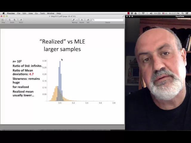
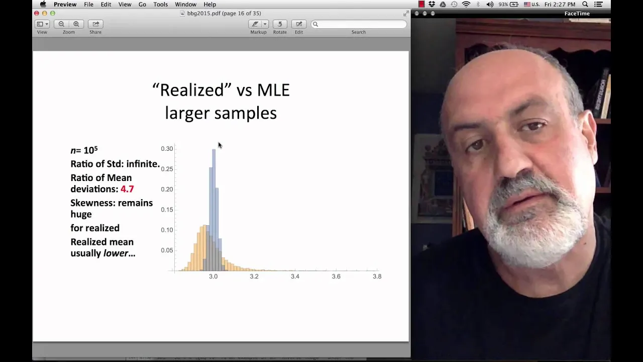
It's actually a very stable some transition. Uh if I take a larger sample remember we said before that the convergence happened at uh square root of n. We saw it from the speed like you're adding information and uh uh and when the alpha is low of course it happens very slowly if alpha is one no information will add it no observation will add information so look when you start increasing the sample this of course converges at root n and the other ones doesn't so the difference between them is huge so here I have uh 100,000 uh n and look at the difference between them and of Of course, if you go to a million, it's going to be a lot bigger.

Simple conclusion. You cannot use the mean to estimate the mean. That is a no no.

And I'm saying I'm using statistical theory. Okay, you cannot there's no you cannot estimate the mean uh use the mean to estimate the mean in for a power law. Okay, that's a no no.

Uh you can show analytically from here uh uh that that this is a great estimator. Okay. Whether you use alpha distributed as log normal or normal, it doesn't matter much.

Uh next we're going to have a uh something more interesting. Okay, with alpha less than one, they are cases that effectively appear to be power laws, but they have a little hitch that allows us to see the mean. So to see the difference between observed mean and realized mean case study in violence that I did with Sher Lo here you can see in this one the difference between observed mean okay and theoretical mean the true mean okay or the estimated mean you see the this one will be lower than that one okay and of course the lower the alpha the more wedge between them and this effectively allowed us to work with an alpha 55 0.

55 very very low alpha from a mistake I I made uh early in my uh in my career in power laws I was under the belief that when something has an infinite variance okay so and and or something has an infinite infinite moment that that effective because it's unbounded if you put a boundary say for example now we're dealing with violence uh no event can be uh can kill more than 7. 2 two billion people. I know it's very remote boundary but you can still put it there.

I thought that some if the the mean was infinite that it would be 7. 2 billion and and uh that was my intuition and and effectively but moment thought the same and I realized nobody made the calculation of hey you know what if we had a distribution that acted like power law on the transformation but transformed back into compact support. Okay, what would be the mean?

Would it be on a high here? So if I have LH lower bound L higher H which is a copax support of the true distribution of violence u L can be arbitrary set 5,000 10,000 whatever you define as violence uh you know as big violence under consideration and H is the exact u uh maximum number that violence can kill. So it's really technically unbounded not technically but but it has it has a mean.

Okay. And that we do a transformation of fi into something that has uh remove the compact support on one side. Uh phi has to satisfy some condition.

I use this one. You know people in finance do it all the time. We have stock prices can be between zero and infinity by taking log of uh prices of relative prices.

Then you open it up on the left side. So you do from you're on a real line minus infinity to infinity. we can perform analytics on power law and then come back we convert back and they of course got to be the same parameters that's the beauty of just like in finance whether you work with normal log normal it's the same parameters but they mean different things and different distribution uh and look we got beautiful fit I've never seen anything like that uh for the near tail which is my department and who deal with extreme got a beautiful uh uh performance on a far tale that's for violence I'm not going to uh I'm not talking about violence.

It's more this is more of a methodology thing. And this allows us to to compare the true mean to the sample mean because again let's take these distribution. They have something very weird that they're they're dominated by rare events and these rare events are rarely in the sample because the right tail is not seen.

So and I discuss it at lengths in the black swan. People don't typically get it until I draw the graph or show them the mass is that 96% of the observation for example something like this are going to fall below the mean. So odds are when you observe a sample it's going to underestimate its true mean until that observation comes to you know put it back in place.

So uh it's just like in finance you know you observe you observe you observe until the crash right you don't have an idea of how bad things can be on the left. Uh so so that's a nice exercise where working with a distribution of alpha and you can stocasticize alpha and look at the range of alpha you can get an idea of the mean okay the second point let's apply this to pikat thing I mean I I love the idea of of inequality is not good and stuff that's not the point the point is methodology okay that uh and I start smelling people start talking about centile contribution okay sile contribution hey you guys are talking about a mean and they're accepting that it's a power law and they're expecting there's concentration they're accepting fat tail just like with a pinker fellow he accepts it's a power law somewhere whatever and then the other patient start talking about changing the mean they're making a of course it's very small mistake compared to the just making journalistic mean but still there's a problem there so I smelled it and uh and just got on my computer and did the moniko and of course did some analytics with Rafael Daddy And uh uh we discovered the following. If you observe 8020 which by recursing uh gives you top 1% has 53%.

If that's what you observe effectively the top 1% would have more like 75%. It's just that the way you measure it from the the the average the okay the the the percentile contribution you say the top 1% had the share of the total means you're taking the mean for that conditional mean as we do here you take that conditional mean divided by the total mean okay it's how it's really done so we're taking a ratio of two means one conditional one unconditional that's a quantile contribution you're definitely going to have that bias simply because you know the mean is not a variable for for uh for for these things the location of the distribution maybe variable but not okay so and this is a bias okay if I have a sample of a thousand at the true ratios that the top 1% should have 65% 66% of the total the mean all right the LC the variable will be 04 so we'll have a huge estimates of 0. 25.

You see why that's the problem with the distribution and uh and then when you go to 100 million in your sample you still have a huge bias and not a sample in your population. It's what that that's the situation. But when you go via the alpha, you estimate the alpha, you don't have that bias.

Again, this is strange. The same applies to what's called geni coefficient. Uh this is a coefficient also drink.

The genie coefficient again you're talking about relative mean sorry not the difference the mean difference uh absolute difference between all your variables. And if the genie is one it means you have maximum inequality. If the genie is uh if the genie is uh uh uh z closer to zero uh it means that everybody's making exactly the same amount of money.

Um so and then these are the two ways they measure the genie measure. This is the theoretical this is the uh the thing here for a power law that's a genie. The genie comes you know has distribution from the alpha pole distribution and effectively when the true genie is 0 83 and you look at the small population you get 75 a huge bias and then as your population increases as with PKT you're going to see more inequality that's just the the system so the the the I will stop here we can continue now in a second moment because you know as I said no one uh thanks uh the the the finally let me say something.

I am not saying that measuring the way we're measuring is uh going to give you a perfect answer. I am saying if you are going to do statistical inference these are the variables to to work with. things can be more complicated under uh conditional alpha under all these that's fine but if you're gonna work with something work with the alpha okay if you work with uh the wrong variable you're going to get the wrong answer is very prevalent actually in the end here I have I'm going to skip this section here that much of finance social science relies on bogus estimators and no wonder why when we talk about volatility you have to recalibrate models because they're not estimators chasing past fitness.

If you had to rec, you know, we don't recalibrate the speed of light. But in social science, they keep recalibrating something. Why?

Because they have the wrong variable. They once every day recalibrate their models. It is offensive.

See, so they're chasing past fitnesses. As the late the great Benov said, when lightning hits, we do not change the law of nature. Right?

Uh should be the same. uh you should the the you know calibrate the speed of light there make few mistakes maybe and then you zoomed in on it and that's it now converge to so it should be maybe not the same but your calibration error over time should decrease but here no we still have the difference between calibrated model and delivered doesn't seem to shrink which is why most of social sciences is largely particularly when you deal with micro now excellent news is that rigorous methods extreme value theory can help us get closer Again we're not getting very close. One more thing I want to add here is that when I look at these classes of distributions if you think things I want to add when you look at these distribution you have to remember that things fool you uh downwards not upward.

In other words uh a power law can disguise as a Gaussian in small samples but a Gaussian cannot disguise itself as a power law. I call that in black swan the masquerade problem. in and here I showed it I I talked about the tail dominance.

Um something that delivers a jump of 500 standard deviation cannot possibly uh Gaussian. Okay. So uh so you cannot be fooled by a power law.

You can be fooled by a Gaussian. So there is some kind of dominance in the way you select your distributions. Thank you friends.