Statistical Learning: 6.6 Shrinkage methods and ridge regression

foreign welcome back so we've talked about a fourth stepwise selection backwards stepways in all subsets as well as some techniques for choosing the model size all those methods fit by least squares so whenever we consider model a subset we always fit the coefficients by least squares now we're going to talk about a different a different method called shrinkage namely two techniques Ridge regression and lasso and as we'll see that these methods do not use fully squares to fit but rather different Criterion that has a penalty that will shrink the coefficients towards typically zero and we'll

see this can be these methods are very powerful in particular they can be applied to very large data sets like the kind that we see more and more often these days where the number of variables might be in the thousands or even Millions so um and one thing that's worth mentioning is that like Ridge regression lasso and shrinkage messages like this are a really contemporary area of research right now I mean there's papers every day written by statisticians about variants of these methods and how to improve them and that sort of thing as opposed to

some of the other things that we've covered so far in this course where you know the ideas have been around for 30 40 years although actually for Ridge regression I think was evented in the 70s but it's it is true that it wasn't very popular for many many years it's only sort of what the the Advent of fast computation in the last 10 years that it's become very very popular along with the lasso so um some of these methods are old some are new but they're really quite hot now in their applications so Ridge regression

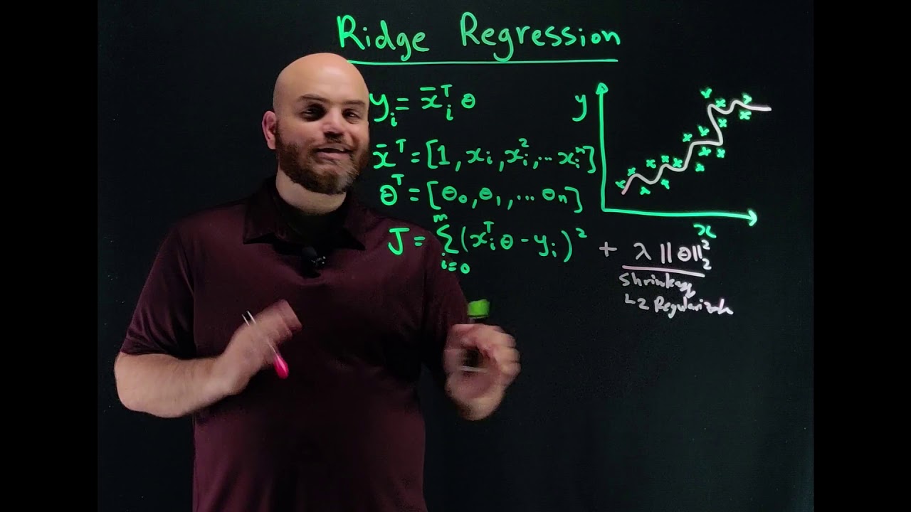
now let's first of all just remind ourselves what least squares is the training error um so the RSS or training error is the sum of squares deviation between Y and the predictions so when you do these squares we simply find the coefficients that make this as small as possible now with the rich regression we're going to do something a little bit different we're going to use training error RSS we're going to we're going to add a penalty to that namely a tuning parameter which will choose in some way and you'll as you can guess it'll

be back cross validation times the sum of the squares of the coefficients so this we're going to try to make this total quantity small which means we're going to try to make the the fit good by making the RSS small but at the same time we're going to have something which is going to push us the other direction this is going to penalize the coefficients which get too large right the bigger the the more non-zero coefficient is the larger this is so we're going to pay a price for being non-zero it'll pay a a bigger

price that the larger the coefficients are so it's it's basically Fit versus the size of the coefficients and that penalty is called a shrinkage a shrinkage penalty because it's going to encourage the the parameters to be to be shrunk towards zero and the amount by which you're encouraged to be zero is is it will be uh determined by this this tuning parameter Lambda if Lambda is zero let's go back to this if lambda zero of course we're just doing least squares right because this term will be zero but the larger Lambda is this tuning parameter

the more and more of a price will pay for making these coefficients non-zero if you make Lambda extremely large then at some point the coefficients are going to be very close to zero because they'll have to be close to zero to make this this term small enough right no matter how good they help to fit we're going to pay a large price in in um in the penalty term so in other words This this term has the effect of shrinking the coefficients towards zero and Y zero while zero is a natural value remember zero of

course if a coefficient is zero the feature is not appearing in the model so it's if you're going to shrink towards some value that a zero is a is a is a natural place to shrink towards and the tuning parameter the side swing parameter it trades off the Fit versus the size of the coefficients so as you can imagine the choosing a good value for Lambda for for extreme Prime Lambda is is critical and cross validation is what we're going to use for this so let's see what happens for the credit data um well let

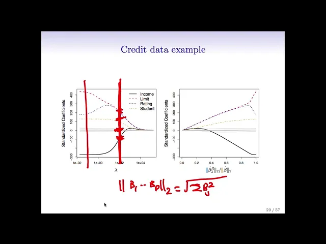
me just go back here so if we think of this for a fixed value of Lambda we have to we have to find the smallest value of this Criterion and again it's just an optimization problem with actually a very simple solution and there are computer programs for doing that so I've used such a program and we'll talk in the actually in the r session about an R function for doing Ridge regression but let's see what it looks like in this example in the credit example so here we've plotted the coefficients um standardized coefficients versus Lambda

for the credit data and let's see what happens well first of all on the on the left hand side Lambda is close to zero so there's almost no no constraint on the coefficients so here we're pretty much getting the full least squares estimates and now as Lambda gets larger it's pushing the coefficients towards zero because we're paying more and more of a price for being non-zero in the extreme over here where Lambda is a little more than are maybe more than ten thousand the little coefficients are all essentially zero in between they're shrunken towards zero

as Lambda gets larger although not not uh uniformly so right like this the rating variable actually gets bigger for a while and then shrinks back down to zero and I remember when I was a student figure again and again actually was in a class that Rob was teaching and being totally confused and Futures so I just want to spare everyone this confusion in case anyone shares a confusion I had so like if we look here this red line indicates the spot at which Lambda equals 100 and at that spot the income coefficient takes on a

value of like negative 100 these other six coefficients here are all around zero student takes on a value of around 100 limited rating take on values of around 250 and so the point is what we're plotting here is a ton of different models for a huge grid of Lambda values and you just need to choose the value of Lambda and then look at that vertical cross section good and is so as Danielle said if we chose the value of Lambda about was that a hundred then it would seems like it chooses about three non-zero coefficients

the black the blue and the red oh maybe four and then these guys here are basically essentially zero the gray ones so they're not quite zero but they're small right exactly so an equivalent picture on the right now we've plotted the um the standardized coefficients as a function of the of the the L2 Norm the sums of the squares the square root of the sum of the squares of the coefficients divided by that the L2 Norm of the fully squares coefficient so Rob what's the L2 Norm okay um the L2 Norm so the L2 Norm

of the beta of the vector beta 1 through beta p it's written this way or the so the L2 Norm so it's the square root of the sum beta J squared all right so this is the that's the L2 norm and so it's synthesis that's it so um we see here when the L2 Norm is zero so when the coefficients are all zero the L2 Norm is zero that corresponds to the the the right side of this picture so the Lambda is very large here it's large enough that it's driven the L2 normal down almost

to zero so the coefficients are basically zero and then on the on the right um Lambda is very small and we get the full least squares estimates and in between we get again a shrunken coefficient so these two pictures are very the same but they've been flipped from left to right and the the x-axis are parameterized in a different way so Rob why does um this x-axis on the right hand side go from zero to one why does it end at one oh because we just we plotted the stat it ends at one because we're

plotting as a function of this standardized L2 Norm so at the right hand side um we get we have the basically the full lead squares estimates so these numerator and denominator are the same right so on the right hand side here on this right hand plot Lambda is zero and so your Ridge regression estimate is the same as your least squares estimate and so that ratio is just one exactly okay um I think we've actually just said all this thanks for the questions from Daniella um right so there's the L2 Norm defined I wrote it

in the previous slide and that's what was used for the plotting axis um one important point with Ridge regression is that it it matters whether you scale the variables or not now just just to remind you if you just do standardly squares so starting these squares is called scale and variant If I multiply a feature by a constant it's not going to matter because I can divide the coefficient by the same constant I get the same answer so in least squares the the scaling of the of the variable that doesn't matter so whether I measure

a length in feet or inches it's not going to matter because the coefficient can just account for the change in units but it's a little bit subtle here now for for Ridge regression and penalized methods like rage regression the scaling does matter in an important way and that's because if we go back to the definition of ridge regression right these coefficients are all put in a penalty together and they're this there's a sum of squares so if I change the units of one variable it's going to change the scale of the coefficients well if I

change the units of one variable the coefficient has to change to try to accommodate for that change but it's competing against the the coefficients for other features so because they're all put together in a penalty in a sum the the uh the scale of the features matters and as a result it's important to standardize the predictors in regression before applying Ridge regression so in most cases before you do a ridge regression you want to standardize the variables what does that mean to standardize the variables well you take the the variable or feature and you divide

it by the standard deviation of that feature over all the observations and now the standard deviation of this guy is one and you do that for each feature and that makes the features comparable and makes their coefficients comparable so that's an example of Ridge regression compared to least squares here's a simulated example with 50 observations and 45 predictors in which all of the predictors have been given non-zero coefficients so we see on the on the left we see the um the bias in Black the variance in green and the test air in purple for Rich

regression as a function of Lambda and the same thing on the right as a function now of the standardized coefficients of the sorry of the of the two Norm of of the average regression divided by the two over fully squares so again these are the same pictures essentially but the the x-axis have been changed let's look over here we can see that um what happens while the the bias as we move so fully squares is is over here on the Left Right Lambda is close to zero as we as we make Lambda larger the bias

is pretty much unchanged but the variance drops so so Ridge regression by shrinking the coefficient towards zero controls the variance it doesn't allow the coefficient to be too big and it gets rewarded because the mean square error which is the sum of these two goes down so here's the here's the place where the mean square is minimized and it's lower than that for than the fully squared estimate so in this example Ridge regression has improved the error the the mean square error of fully squares by shrinking the coefficients by a certain amount and we see

the same thing on in this picture and actually this U-shaped curve that we see for the um the mean squared error in this figure in purple comes up again and again where when we're considering a bunch of different models that sort of have different levels of flexibility or complexity there's usually some sweet spot in the middle that has the smallest test error and that's really what we're going for so that's what's marked as an X in these two figures so I want to go back to this picture of Ridge let me clear the and one

thing you might have noticed here that we mentioned is that the coefficients are never exactly zero they're close to zero like here these gray guys are all closer but they're they're never exactly zero matter of fact you can show mathematically that they're unless you're extremely lucky you're not gonna get a coefficient exactly of zero so Ridge regression shrinks things in a continuous way towards zero but doesn't actually select variables by setting a coefficient equal to zero exactly but it seems like a Pity in this example right because all those gray variables are so tiny it

would just be more convenient if they were zero right which is a great setup for the next method called the lasso