Probability

well hello Internet and welcome to my probability course in this one video you're going to learn pretty much everything you could learn about probabilities from a 500 page textbook it includes numerous formulas with real world examples that demonstrate every single formula and if you pause your way through it and take notes you will have a solid understanding of probability on a very deep level and if there is a lot of interest in this tutorial I will continue to create one for statistics linear algebra and calculus and completely cover the math of machine learning so probability basically focuses on finding the chance a random event will occur over the long term probability is a number between 0 and 1 but also is represented by percentages and a basic probability can be found by dividing your preferred event by all of the other possible events for example coin flip has a 0. 5 probability of coming up either heads or tails now to find all possible outcomes if you would roll two dice what you would do is multiply 6 times 6 to get a total of 36 and you can see here all of the probabilities of rolling two dice now this is a very important slide to understand because I'll be using it many other times across the course of this tutorial in multiple different examples now if you see the symbol PA this simply stands for the probability of the event a occurring a set is going to be a list of all possible outcomes and if we decide we want the union of two sets we create a set that contains all values in either set and you can think of the word Union as being similar to the word or and you can see here is the symbol for Union and if the value is in set one or set two it is of course going to be part of the Union of those two sets an intersection which is like the union symbol flipped upside down whenever it is used with two sets will contain only values in both sets and like the union the intersection is going to act like an and condition so you can think of the intersection symbol as the word and meaning that the values are in both sets so for example and then finally if you have a with the values 1 3 and 5 and a set with all values from one through five the complement of a would be two and four because those are the values that are not in set a now conditional problem abilities deal with how probabilities change given other events occur for example what is the probability that a die roll is five given this symbol means given that we know the die roll is an odd number to find the answer all we do is divide the probability of rolling a 5 using a six-sided die which is given a probability of one-sixth by the probability of rolling an odd value which has a probability of one-half and whenever we do that we see that given we know the value is odd there is a one in three probability of rolling a five now let's use the conditional probability formula again let's say I have data on 200 men as well as women who exercise or not now if I randomly picked a person that exercises what is the probability that that person is a woman to find this I take 17 over 200 representing the women that exercise and divide that by the total people who exercise which is going to be 39 over 200 and if I do this I find that there is a 43. 6 percent chance that if I pick a person that exercises that that person is going to be a woman and this over here is called a contingency table and it contains all of the probabilities depending on multiple different outcomes and intersections between the rows and columns provide joint probabilities between those events now in this example what I want to do is I want to find out if a randomly chosen person is a woman or an exerciser and for this we're going to use what is called the addition Rule now if two probabilities are exclusive we are going to add them but in this case it is possible for someone to be both a woman as well as a person that exercises so to find our answer I must subtract out the intersection of women as well as exercises and you can see that subtraction taking place right here and so as you can see there is a 0.

61 probability that a random person will be a woman or an exerciser and this is an example of what we call a joint probability because we are looking for a person with two characteristics if we said we wanted to look at exercises and then from that group pull out just women that would be an example of what we call a conditional probability now probabilities can be either dependent or independent meaning whether they affect each other and to find dependence we want to find if the probability of a given B remember this line means given right here as well as this is going to be equal to the probability of a and vice versa so if they are dependent and so in that situation they would be dependent so if we know that the probability of a die being odd affects the probability of a dice roll and we see dependence however a die being odd doesn't affect the probability of a die roll for either an even or odd dice roll now you're going to find probabilities of independent events and dependent events in different ways now if an event is independent what we're going to do is multiply their probabilities for example to find the probability of rolling a 1 and then a two both who have a probability of 1 and 6 or 0. 167 we're going to multiply them to find a probability of 2. 8 percent mutually exclusive events however can't occur at once so with them you add their probabilities so to find the probability of rolling a one and then an even number with two dice what we're going to do is add 1 6 plus one half to get two-thirds and as you can see that makes sense because 4 values out of six is equal to two-thirds in this situation now Venn diagrams can be very useful for representing events and how they interact they work best for marginal probabilities being probabilities that don't affect each other and they also work in very well with joint probability abilities which measure the likelihood of events occurring together they don't however work well with conditional probabilities and when analyzing sequences of events and you can see here all the symbols you have seen so far work together in one Venn diagram and down at the bottom of the screen right here where we have the C this is going to represent the complement of the event and here what I'm going to do is use our previous exercising table in a Venn diagram format and you can see how the table data translates over from our table into our Venn diagram now tree diagrams are normally used whenever Venn diagrams cannot be used and they work best with multi-stage and conditional probability problems which is the opposite versus the Venn diagrams they however work poorly when events take place at the same time and here what I'm going to do is break down the process of flipping a coin twice and you can see that we can find just by using this tree diagram that that probability would be 0.

5 for each of the individual coin flips and 0. 25 whenever we include both coin flips here also just to cover something a little bit more complicated looking is a tree diagram that's going to represent the different toppings you can have on a hamburger in this situation you can see that there are 16 possibilities with a one Burger option which of course would double by adding another Burger to our equation and as we continue we'll get into ways that this can be more helpful whenever we deal with things called permutations combinations and variations now here what I'm going to do is find the total probability based off of two options to find it what we're going to need to do is sum probabilities where we multiply the probability of a given B by the probability of B now in this example we have two options of brake pads of differing quality you can see here brake pad X is going to give us 40 000 miles 95 percent of the time and they control sixty percent of the market while brake pad Y is going to give us 40 000 miles 92 percent of the time and they include 40 percent of the market and what I want to do is calculate if I buy a random brake pad that it is going to last forty Thousand Miles now we find the probability of a random purchase allowing us to travel forty Thousand Miles and we can see here that that works out to 93. 8 percent and any time you want the marginal probability of multiple different events that are identical what you'll know what you will know that you are looking for is what is called the total problem ability and here just to reinforce this as another example if I know the satisfaction ratings and the percentage of market share owned by different car insurers I can find the probability that I will be satisfied with my car insurance and all I need to do is add up those values taken from here this being the percentage of market share owned by each of the different companies and over here where we represent the percentage of customers that are satisfied or dissatisfied add all those up and get 86.

97 percent now Bayes theorem is going to be used to find a probability when we know other probabilities and it comes in two forms in which I will demonstrate both of here's one form here's the other form here I'll find the probability that if I know I have an exerciser meaning a person that exercises what is the probability that they are a man now I'll take the data from our chart and then I plug it into base to get a result of 0. 564 and then I can double check my work by finding my results equal 22 over 100. now I'm going to use another form of Base here if 3.

98 of people are infected with a disease and 98 with the disease test positive and there is a one percent false positive what is the probability that I'm in fact if that I am infected if I check positive well to figure this out I multiply the probability of infection by the probability of testing positive given that I am infected and then I sum the product of infected as well as positive tests by the product of non-infected by false positives I then divide and find that there is an 80. 9 percent chance that I'm infected based off of errors in the test and the low probability of people that are infected now the Bayes theorem is super super useful so I want to give you another example of how we can use it here we have three toy manufacturing machines and each is going to make different quantities and a known percentage of flawed toys and what I want to do is figure out if I know a toy is flawed what is the probability that it was made in this example by Machine C now here x will represent the event that machine a b or c made it y then is going to represent the probability that the toy is flawed based on the machine and I'll then find the sum of X multiplied by y for each machine and I'll find the product of flawed toys from C by the percentage of toys made by C and then and you can see here after I divide I find that there is an 11. 69 percent chance C made the toy if I receive it and it is flawed now moving on combine a Torx is going to be concerned with the number of ways items can be ordered and they include permutations variations as well as combinations permutations focus on the number of ways items can be arranged and you find them basically just by taking the factorial for example there are 24 ways to arrange four items and we find that by multiplying four times three times two times one and you can also see in the pictures on the side how those break down now you're going to be able to find the number of permutations of X items chosen from a list of n items as well once again you're going to use the factorial and you can see the formula that we have right here so in this example if you were picking three runners for a relay race from a group of five you'd find that that is going to provide 60 permutations however maybe a more interesting example would be what is the probability of drawing the numbers one to five out of a possible number of 15 numbers now to save time you can also come in here and cancel out the factorial of 10 from the top as well as the bottom to get 360 360 permutations and then if you would go on to divide one by that number you find that it is extremely rare which would come out to point zero zero zero zero zero two eight now when calculating combinations the order is not going to matter and here I'm going to cover combinations without repetition and this means a value can only be used once you can see here here the formula that you are going to use to calculate the combinations where X is going to represent the number of items Chosen and N is going to represent the total available number of items to pick from and whenever we calculate the number of combinations when we want three numbers from a group of 10 without repetition we find that we get a value of 120 so there's 120 combinations if we Define those rules and follow them we can also find combinations with repetition and you can see here the same exact formula we had before where n is the number of items to choose from and acts of the number of items to pick this time we're going to calculate the number of Lottery combinations with repetition and we can see that the total number of combinations jumps up to 220 because after we go and pick a ball we throw it back in we dramatically increase the odd so we could pick it again now what I'm going to do is analyze the number of possible winning hands we can expect in a game of poker and just to make sure you're aware there are 52 cards in a deck of poker cards and there are four different suits Hearts Spades clubs and diamonds as well as two different colors being black and red in this example what I want to do is calculate the number of possible hands that provide four of a kind and we're going to start off with the total number of Suits being four then what we're going to do is pick the number we want four of a kind of from a total of 13 possible cards Ace the whole way up through king that's thirteen cards and of course there are 13 cards for each suit now since we picked our value we want four of a kind of and we have that card for each of the four suits we now must pick our fifth card and there are only 12 cards left so what we're going to do is multiply times 12 and then finally to finish off we must decide on the suit of our fifth card and after we multiply all of the above together we are going to find that there are 624 possible ways to create four of a kind in a game of poker now whenever we are calculating the total number of Full Houses we must use our combination formula and the very first thing we're going to do is to pick the value we want 3 out of a possible 13 cards then we want to pick what we want two of out of the remaining 12 cards and now there are three ways out of four to pick the suit for our first three of a kind card and we're going to use the combination formula to find four total combinations then we are once again going to use the formula to find six combinations when picking the suit for our pair of cards and then what we do is multiply those together and we find that there are 3744 ways of getting a full house in the Game of Poker we can then once again go in and divide by the total number of possible hands in poker which is that big number you see down there in the lower right hand corner and we can see that the probability of being dealt a full house is .

14 now very often you will come to the question of exactly which should we use well basically permutations are going to be used with an equal number of elements as well as positions combinations are going to be used when you only care which elements made it and variations are going to be used when there are more elements than you have positions so to provide another example let's say we want to find out how many possible values we can use to unlock a combination lock we take the number of elements to the power of the number of positions to get one thousand and this is going to be done whenever we have repetition as a possibility when you don't want repetition you're going to use a completely different formula and here what we want to do is find out how many variations of Pokemon cards can you create if you pick three cards from the total of five and if we plug those numbers into our formula you can see that our final result would be 60 variations now random variables are going to represent the results of your calculation and there are three types being finite and you can see here in an example of a finite variable the number of sixes rolled in a thousand throws we're also going to have countably infinite which would be as if you would count the number of sixes rolled over the course of a year and then you have uncountable infinite which would be the number of sixes rolled on the entire planet Earth and now we're going to talk about something called discrete uniform distribution now a probability Mass function is going to assign probabilities to random variables now you know that a six-sided die in any one role has a probability of one-sixth and the most basic probability model is known as a discrete uniform distribution an example would be a single die roll or a single coin flip now to be a discrete uniform distribution all possible values of X must be consecutive integers like 1 through 6 with die rolls and each value 4X must have an equal probability of occurring and to calculate the probability mass of a die roll what we're going to do is just simply take 1 over B minus a plus one where B is going to be the maximum value and a is the lowest value and for for a die roll that is going to equal 1 6. now variance is going to measure how far a set of numbers is spread out and to calculate that you're just going to take B minus a plus 2 multiplied by B minus a divided by 12. where again B is the maximum value and a is the lowest value and with a die roll we can see that that works out to 2.

9 or 3. now with this chart you can see that it's going to provide the probability mass for each roll of 2 dice a relative frequency histogram is going to show how often values are expected for each roll of those two dice and this is what is called a cumulative distribution chart which is going to provide the cumulative probability associated with adding additional possible dice rolls you can see here as we add those the percentages go go up until we get here finally to one which would be one hundred percent now the expected value is going to be the long term expected average and it is found by summing all multiples of X by the probability of X so for our dice rolls that works out to 6. 985 or 7.

you can see over here that 7 has the greatest probability of occurring whenever you throw two dice now calculating variance with multiple variables is a bit more complex to do so what you're going to do is sum the total of all values of x squared and multiplied by the probability and whenever we do that we get a value of 54. 645 then what we will finally have to do is subtract from that the square of the expected value calculated previously to get a final value of 5. 8 855 now the standard deviation is going to be a measure of the amount of variation and if that number is low it means it is close to the mean average if however it is high that means it is going to be spread over a very large or wide range and to find it you just take the square root of the variance which in this situation would work out to 2.

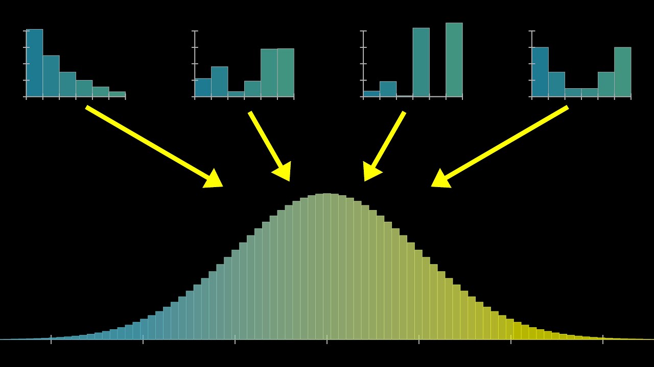
419 now with a normal distribution in which we contain 100 of the probability under the curve we also have an equal bell curve with the same area under both sides we also are going to see here that the mean and median are going to be equal and we also see that 68 of the total area is one standard deviation from the mean this then is going to continue with 95 percent being contained under two standard deviate Asians and 99. 7 percent for three standard deviations and this is known as the empirical rule the empirical rule says that one standard deviation equals 68 percent two equals ninety five and three equals 99. 7 and I further break that down here into all the different parts for all standard deviation distributions also notice that just point three percent over here or point one five percent on both sides is all that is left after three standard deviations and that brings us to Z scores the z-score is going to give us the value in standard deviations for the percentile we want and an example is going to make this very clear so for example if we want 95 of the data it's going to tell us how many standard deviations are going to be required and the formula asks for for the length from the mean 2X and then divides by the standard deviation and now with this example it'll all make sense so this is a z table on the right side of the screen and if we know our mean is 40.

8 as you can see down here the standard deviation is going to be 3. 5 and we want the area to the left of the point 48 so we want all this area we perform our calculation to get 2. 06 we can then find 2.

0 right here there's the 2 and then across the top we can find 0. 06 which is right here and this is going to tell us that the area under the curve is going to make up 0. 98 or 98 of the total area we can also find the area to the left of the mean with a negative Z table so if we want to find find the area left of 36.

3 with a mean of 40. 8 we perform our calculation to get Negative 1. 29 we then look up negative 1.

2 and 0. 09 in the negative Z table and we see that our answer is 0. 09853 so the area under the curve from that point to the left is .

098 now let's go completely in Reverse let's say I want to calculate the score I must get to score in the top 1 percent of my class now I know the mean is 0. 79 and the standard deviation is 7. 5 I then look for 0.

99 which would represent top one percent in the Z table to find the z-score of 2. 33 2. 3 right there and 2.

3 right there and 0. 99 which is right there then if I plug that into our formula and so solve for x I find that I must score 96. 48 to place in the top one percent of my test based off of all the supplied data now we have been using Point estimates so far which represent a singular point of data and the mean would be an example of a point estimate now while Point estimates are easy to calculate they can also be very inaccurate at times and an alternative is to use a what we call an interval or a range of values so if I have three sample means taken from three different data sets I can create an interval that covers their range of different values I then have to find how confident I am in that interval and we normally Define normal confidences as 90 95 or 99 and this is going to mean that if we have a confidence of 90 percent that we expect 9 out of our 10 intervals to contain our mean value now when calculating our interval what we do is we take our sample mean and find the values of X and Y by adding and subtracting the margin of error Alpha is going to represent the doubt that we have so if we have a confidence of 90 percent then in that situation the alpha would be ten percent n is going to represent our sample size and we were going to use once again a z table to find our interval so in this example I've gathered all of our data and if we look up 0.

025 on our Z table we get a value of 0. 508 and if we plug that data into our formula we find that X is going to equal 42. 97 and then once again we can also find that Y is going to equal 43.

029 and now we will move on to cover binomial probability and it mainly is going to focus on whether we will or won't have a successful event there are however conditions if you want to use this formula first off you must have multiple fixed trials with an outcome of pass or fail the outcome of each trial can't affect any of the other trials and then finally the probability for each trial must be equal so for example if you are rolling one die 100 times and want the binomial distribution of rolling a six that is okay mainly because you met all of our conditions however rolling a dice until you get five sixes doesn't apply because the number of Trials is not fixed here is the binomial probability formula and you can see that n is going to represent the number of Trials or the number of successes and we must find the number of combinations and P is also going to represent the probability for each of those values so what I want to do here is calculate the probability of getting exactly four sixes in 10 rolls first we have to find the total number of combinations and this is known as the binomial coefficient then we plug in the values and we find that our probability is 0. 048 and as we analyze our formula further we can see the parts representing the probability of success as well as the probability of failure now poisson distributions are going to focus on the probability a specific number of events will occur over time or distance or area for example the number of visits to a website per day or hour the number of pizzas sold the number of red cars seen vegetables expected for Harvest and so on now the conditions to use this are going to include that you count occurrences over time distance scenario the mean occurrence must be the same over a similar time area or distance the count occurrences over an interval can't depend on other intervals and intervals can't overlap in this example if we can grow six heads of lettuce in 0. 3 square meters what is the probability we can grow eight now Lambda is going to be equal to 6 and if I plug in my values I get .

103 or 10. 3 percent and as you can see the more X diverges from Lambda the lower the probability it is important to make sure that X has a value no lower than zero and then if you want to find the probability of getting at least eight heads of lettuce we're going to sum the probabilities for zero through seven and then subtract one we now move on to geometric probability which is is going to be used to calculate the probability of success depending on the number of trials for example how many dice rolls are required to get a six now the conditions for using it include that trials must be independent outcomes are going to be either pass or fail probability of success must be constant and the number of Trials need not be fixed like with binomials and as you can see we are multiplying the probability of success by the probability of failure to the power of the number of Trials minus one now to find the probability of rolling a six in three dice rolls what we're going to do is multiply the probability of a roll which is 0. 167 or 1 over 6 by the failure probability which is going to be 0.

833 1 minus point 0. 167 and this is going to be taken to the power of the trials -1 like we saw previously and you can see that that is going to come out to 0. 116 and then if you want to find the probability of success in three or less rolls what we're going to do is sum all previous process probabilities which is going to work out to 0.

422 now we can also find the probability that it will take more than three dice rolls simply by subtracting the previous probability from one and we can calculate how many dice rolls it will take to get a success in this situation and this is going to be called the mean and we can see success is expected in approximately six dice rolls and I'm also going to show here how to calculate both variance as well as standard deviation and you can see those formulas right here and this represents a square root now I want to briefly talk about sampling whenever we are gathering samples it is important to follow the central limit theorem now the conditions of it are that samples must be random the samples must be representative of the population and that you use sampling with replacement or that you sample less than 10 percent of the total population and now we're going to go on and talk about negative binomial probability now while the geometric model is going to find the number of Trials required for success or the number of dice rolls before you get a six the negative binomial model is going to find the number of Trials until the nth success so for example how many rolls are required until you get three sixes now the conditions to use this are that you must have independent random trials with either a pass or fail for all of the trials the probability of success is going to be equal for each trial and then finally you must keep track of the number of Trials up to the Target success now very often the most confusing decision is based on which formula you should use and when now the binomial model is going to be used when you want to count the number of successes with a fixed number of Trials the negative binomial model however is going to count the number of Trials required to find a fixed number of successes and then finally the geometric model is going to be used to find the number of Trials required for one success and here you can see the formula for the negative binomial in this situation p is going to represent the probability of success K is the number of successes I am to have and n is going to represent the number of Trials now let's say we want to calculate the probability of rolling three sixes in 10 rolls well first we have to find the number of combinations by taking 3 from 10 and this is going to be a situation where we will use repetition and that is going to work out to the Number 220 and then we just plug in all of our other values to find a total probability of 28 percent and you can see here our probability of rolling three sixes is going to be maximized at 15 rolls at 0. 354 and then it's actually going to start falling I don't know if you can really see it because it's very slight but it falls dramatically more as we continue and if you think for a minute why exactly that would be well the situation here is that our goal is to get three sixes however at some point we have an increased probability of rolling four sixes which is something that we do not want and that's the reason why it starts to decline after 15. now a hypergeometric distribution is going to be used with samples without Replacements to find the probability a specific number of items is going to fit a defined characteristic with binomial and hypergeometric you're going to find how many people have a characteristic and replacement is going to Define which of those that you are going to use now the required conditions are that you sample without replacement population has an equal chance of being sampled population is also going to be in two groups being those with the important characteristic and those who do not have it as well as the number of people with the characteristic and the total population size must be known and X is going to represent the total number of people you're interested in and here is the formula we're going to used to calculate hypergeometric distribution probabilities and as well I provide a pictogram on the right side of the screen to try to explain the individual parts so this is basically going to represent the whole entire circle here is going to represent the total population then we have with M represented with successes and minus m is failures and then we have our sample being this small circle inside of here and once again the X represents the successes in the sample and again n minus X is going to represent the failures in the sample and here I'm going to work through an example so in this situation what is the probability of getting two black cards if I draw five from a deck without replacement well there are 26 possible black or success cards in this situation and there are two successes in my sample so the total number of cards is 52 for you remember from the number of cards in a pack or a deck of poker cards and then finally I'm going to draw five cards for my entire sample now this is a little bit complicated but it's basically just calculating combinations down here and then bringing everything all together and here is the main formula here but basically if I find the combinations for our formula we have here and work through it you'll see that I have a 0.

325 probability of success of drawing two black cards out of a total of five without replacement and here what I want to do is calculate the expected value which if you don't remember is the number of successes you expect in the sample and whenever I plug in the values I get 2. 5 and then I also will find the variance which again is the average deviation from the mean over the long term and if I plug in those values and work them out you'll find that value is 1. 15 now moving on to understand continuous probability is going to require us to cover a few other different definitions first continuous random variables are going to be variables with an uncountable infinite number of values the probability density function is going to provide the density of the concentration of probability at any point x and continuous uniform distribution is just a continuous random variable used when all the values of the probability density function are the same or are unknown and this variable is going to be between two values being either A or B and this is all going to make a lot more sense with an example so I want to reiterate a continuous uniform distribution is going to be used to find probabilities of success depending on all possible values between a and b and it's going to be used to find probability for an interval rather than a point for example what is the probability that X is between the values of 5 and 6.

I want to cover a couple more things however before I move on to that example one thing to know is the domain of X is going to represent the interval that represents all the different possible values of X and the probability is going to be the area under the curve and this is called the density function of X and some rules that we need to adhere to include that all values of f x must be greater than or equal to zero and also the total area under the curve for all possible values of X are going to be equal to 1. and you can see here is the formula that we're going to use to find continuous probability for X in a given interval and you can also see that you'll be able to find the value of B if you know both the height as well as a and also just to be inclusive here I'm going to provide two just simple examples if you want to calculate probabilities when X is less than 3 or if x in this situation would be greater than 2 which are quite simple to calculate and you can also see on the right side of the screen exactly how we would calculate these areas so if we went from 0 to 4 and so forth and so on and now to finish up everything I want to cover a related topic which is going to be exponential distribution but before moving on to our example I wanted to Define exactly what an exponential function is and simply it is a function of the form a b to the power of X where B is a positive number and X occurs as an exponent an exponential distribution is going to be used for a continuous distribution like we just saw previously in our last example whose probability density has the shape of an exponential function and this type of distribution is very often going to be used to model the time elapsed between events now a density function of the form FX Lambda e to the power of negative Lambda times x where X is greater than or equal to zero in Lambda is constant is going to be representative of this density function and Lambda in this situation is going to be called the parameter of the exponential distribution now a large Lambda is going to cause the slope of the curve to drop quickly to zero and vice versa and like previously the probability of an exponential distribution is going to be the area once again under the curve and you can see here all of the different formulas that we're going to be using for exponentials so less than x greater than x as well as how we will use X or you've calculate this probability in an interval so what let's say that I would want to come in here and I want to calculate the probability of getting home in 15 minutes so if an hour is representative of 1 15 in that situation would be represented with 0. 25 well if I know my mean is going to be represented in which Lambda is going to be equal to 2 where the mean is 1 over Lambda I can just simply plug in these different values into our formula and remember this is a less than situation I want to see if I can get home in less than 15 minutes and if I perform that calculation you could see that I have a 0.

394 chance of getting home in under 15 minutes based off of known information if however I wanted to find out the probability of getting home after 15 minutes using the same data from before and plugging it into our formula you could see that it's much more likely that it's going to take more than 15 minutes being that the answer comes out to 0. 606 and like I said I'm also going to be able to find probabilities in an interval so if let's say I want to find out the probability of getting home between 15 or 40 minutes if I just plug in those values work the calculation you can see that that comes out to 0. 342 and then finally to wrap up absolutely everything if you would want to find the expected value for an exponential all we would do is take 1 over Lambda which is going to work out to 30 minutes and then once again if we would want to find our variance 1 over Lambda squared which is going to come out to one half squared which comes to 0.