Image Intensity Transformation & Spatial Filtering using GDAL & Opencv by Mr. Ravi Bhandari

a very good afternoon to you all all and welcome to the session so this is the sixth six lecture in the series so till now we have discussed about how do we read and write different uh raster formats so today we will discuss about like once after reading reading an image like suppose if you wish to do some kind of processing on that image so basically we will discuss about how do we do some geometric transformation on an image then we will talk about some intensity transformation then some morphological transformation and special filtering on the

images right so till now we had just seen how do we read and write the images now we will see how do we do how do we do how do we manipulate our image right so manipulating the image so that it meets certain application depending on like some applications might be useful for enhancing the visual ization of image some uh operations might be able to remove some noise from the image so like so we will discuss about enhancing or transforming the image like we will apply some trans transformation on the pixels of an image so

that that image becomes more useful for some particular application right so for this anyway I'll be using a combination of open CV and Jal so Jal anyway we have already known so I'll in produce another Library called open CV that that can read and write images as well but plus it is one of the most common use or versatile Library used for uh computer vision applications so basically we will talk about geometric transformation intensity transformation morphological transformation possible and then some special filtering on the images right so if we just recall what an image is

or or uh more precisely Digital Image what is digital image a digital or roster image is represented as we discussed that in multiple lectures a digital or roster image is represented as an array of real numbers right so if you can see that in in image X and y- axis are used to denote the rows and column numbers that are referred as that we said that can be referred as its pixel number line number and pixel number right so all these values these all are pixels and this may be fxy if we say that function

that represents the intensity of that pixel right so X and Y represents its maybe line number and pixel number so any Digital Image can be represented as a two dimensional or three dimensional Matrix of like this there we can say that the pixel intensity is determined by this function f so now the the these all are pixels now we will define something called Neighbors of a pixel right so suppose this is our pixel so there there there can be multiple uh neighbors of this image so one in one instance we can say that these two

pixels on the same line number are the uh neighbors of this or we can specify these two also might be its neighbors so these are two neighbors then these that two diagonal pixels also can be the neighbors or these can be neighbors of a pixel or these all eight pixels can be called The Neighbors ofs of pixel so depending on which kind of application we are referring to so these are the different neighbors of these pixels these can be these four pixels or these four corner pixels right so these these will called two neighbors four

neighbors or eight neighbors of a specified pixel right let now let us talk about Special Operation one of the Special Operations we have already seen that was we were calling at uh local operation of single Pixel operation So Special Operations are performed directly on the pixel of an image right so suppose suppose if you wish to manipulate the the values of our of values of pixels in our image So Special Operations are per being performed directly on the uh pixel of every pixel of every or depending on that so special operations are the operations that

are directly performed on the pixel of image there there are other kind of operations those are called uh frequency domain operations right so those are uh operated uh those those are applied on the for year transform of an image or say in the frequency domain So Special Operations are perform directly on the pixel of an image Special Operations generally can be broadly categorized into three categories right one what we call single Pixel operations or single operation that example we have already seen then other kind of operation Special Operation is called neighborhood operations or focal operation

or then third type of operation which can we apply that is called geometry special Transformations so what is single Pixel operation the value in the output image in is determined by the specified operation on the pixel in an input image right the simplest operation we perform on digital image is to alter the intensity of its pixels individually right so a single Pixel operation means the value of pixel in an out output image is determined by some spe specified operations on on a pixel in a single image or maybe suppose the some operations might involve more

than one images like we may apply the same operation on the uh pixels of more than one image so the value of the pixel in output image is determined by a specified operation on pixel in an input image so the simplest operation that we performed isage to alter the intensity of its pixel individually using some transformation function right maybe it may be multipli scaling by some number or something like supp if you have to app if you are applying this transformation t on the input image Z so that will be calling single Pixel oper so

so this operation will be performed on the every individual pixel right so for example we have seen already like ndv and and ndw at that so we were applying this n minus red divided by n plus red on every pixel of our image the second kind of operation is called neighborhood operation so the value of pixel in output image is determined by a specified operation on the neighborhood of a fixel init in the input image right so in case of single uh single Pixel operation the out the intensity in the output image was based on

just on a single input image right so we are applying some C certain mathematical operation on single input uh input pixel but in case of neighborhood neighborhood pixel the value in the value of the pixel in out output is determined by a specified operation on neighborhood neighborhood pixels of an input image so here will not be the output will not just uh be based on the single Pixel in our input image so it will be based on the we will be applying an operation on the entire neighborhood of a pixel right so depending on maybe

you may choose to apply it on the two two neighbors or maybe eight neighbors four neighbors depending on what kind of application we are doing right so in this case the value in the output uh so supp this was the our XY pixel in our input image then the uh output of XY pixel in our output image will be uh the output of some operation on the all all pixels in the neighborhood of this XY pixel right so like here you can see that it may be like suppose if you are taking this pixel so

when we apply certain operation on all eight neighbor of this pixel so we maybe maybe it may be an average of this entire area or maybe maximum minimum or some other mathematical operation on this entire neighborhood so whatever output comes that output will be assigned to the center pixel op like 21 will be replaced in the output imagees by the value 18.7 so right so that may be an average or maximum minimum or whatever operation we are applying right so in single Pixel operation the out uh the value of output pixel is determined determined just

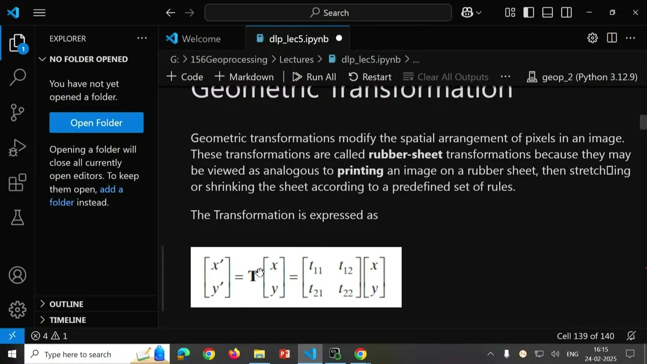
by an single input input pixel but in case of neighborhood operations the output is output is of the output is output we get the output by applying certain operation on the its entire neighborhood right so then then third kind of special transformation is called geometric transformation so these all geometric transformation modify the speciaal arrangement of Arrangements of pixel in an image so till now whatever we were applying those they were are not altering the spatial arrangement of the pixel so geometric transformation is an operation that modifies the spatial Arrangements of a pixel itself like we

may change their locations itself not just intensity we may just change their locations as well so these Transformations are called uh rubber seat transformation because they can be viewed as analogous analogous to printing an image on a rubber sheet then stretching it stretching it stretching shrinking or shet according to the predefined set of rules right so in geometric transformation we are just changing the spatial Arrangements of the pixels as well not just their intensity values we are changing their uh spatial Arrangement as well like this maybe like scaling an image or stretching an image sharing

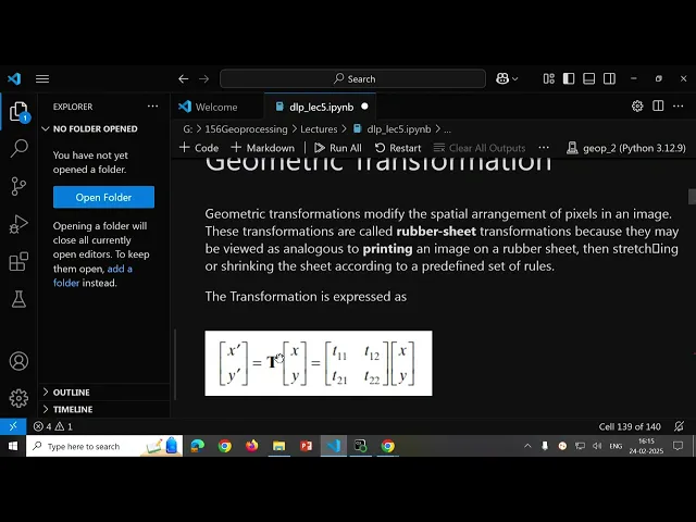
transforming so these are images are operations are called geometric transposition where where we are just modifying it where we are not just modifying the intensity values we are modifying their spatial arrangements as well so any trans geometric transformation can be expressed as a matrix like suppose this was our X X and Y was our original location of our pixel right so we will be applying some transformation on that transformation called t on that XY Vector so then we will be getting new location of that pixel in New Image maybe that might become X Das comma

y Das right so then this transformation can be represented represented as a matrix T of four elements t11 T12 t21 and t21 t22 right so some example of transformation like suppose x d y Das is suppose X by2 comma y by2 that means we are shrinking the origin original image to the half of its size right in both spatial Direction in X and Y Direction We Are if we wish to shrink the original image to by half so that is one kind of geometric transformation it is possible to use like then there are different kinds

of uh geometric transformation like scaling translation rotation or shearing then uh it is possible to use a homogeneous Matrix to express all these operations with a single Matrix right but only their coefficient are going to vary depending on what kind of operation we are doing so these all uh operation like operations of scaling translation rotation and sharing can be represented repres represented as a matrix of 3 cross 3 like so these all will be the elements of that and one we are adding one more row with value 0 0 1 and xy1 so with this

we can perform any of these operations of scaling translation or rotation so what is scaling scaling is just resizing of the image right so the transformation transformation moves the coordinates of pixel of an image to a new location so scaling is just we just wish to resize our image maybe halfing the just we we want to make the pixel size 1 by two or maybe just want to double it to fill the entire screen on and so on so plus the so when we are scaling an image so we need to calculate the values of

pixel intensity in new location right suppose if you are uh stretching our image or reducing or Contracting the image then what happens there will be new locations will be getting like so on the on these new location for these new location we need to calculate new intensity values so the new intensity values need to be assigned to these new locations so this is uh the new intensity values are calculated using something called intensity interpolation so there are most a few common interpolation techniques are nearest neighbor bilinear or by cubic interpolation so in case of nearest

neighbor nearest neighbor assigns the assigns to each new location the intensity of its nearest neighbor in the original image right so the new suppose if you are getting a new location in our transform image then the value in the new location is assigned assigned to the intensity of location assigned the assigns to each new location the intensity of its nearest neighbor in the original image so similarly there are bilinear interpolation it uses the four nearest neighbor to estimate the intensity at a given new location right so the intensity value in a new location will be

calculated based on the four nearest neighbor in the original image similarly in in case of B by cubic interpolation it uses 16 nearest neighbor to estimate the intensity at a given location right now for doing all these operation we will be using uh versatile Library named open CV so open CV they say open CV is the world's biggest computer vision Library open CV is open source and it contains more over 2,500 algorithms and is operated by some nonprofit open source Foundation right open CV is an open source library that includes several hundreds of computer vision

algorithms open CV provides tools for image processing till now Jal whatever as we said that Jal is just a library for reading and writing vector and data formats right so once you read an image using Jal then you get a numpy array now suppose if you used to do some image processing operations on that nump jedar doesn't provide uh those operations so either you can use you can write your own functions or you can use open CV library for doing those image processing tasks right so open CV supports multiple programming languages including C++ python Java

and metlab open CV also is being widely used in various Fields such as robotics robotics augumented reality facial recognition Medical Imaging autonomous vehicles and there are many more areas where it is being used now let us say suppose if you wish to do this geometrical transformation of of scaling on an image right scaling as we have discussed already that scaling is just resizing of the image so open CV comes with a function called cv. resize this resizing can be done done using Jal as well but right now we will be using open CV so open

CV comes with because we are doing many other thing as well so open CV comes with a function called CV do resize for this purpose right the size of image can be specified manually or we can specify a scaling Factor right so either we can specify for orig original image of 100 by 100 cross 100 suppose if you wish to modify it to say 50 by 50 or 2550 we can specify both of these to cv. size either we can specify new new size of the image or we can specify in terms of scaling like

half of that just half make it half or whatever it is then we can specify as we said that because once we are resizing an image there will be new pixel locations for those pixel location we need to calculate new values using interpolation like there are different ways of interpolating new uh values that on those new location so we can specify uh which interpolation technique to be used as well like inter area for inter cubic or inter linear whatever can you specify while spe doing the for interpolation right so for first thing first we need

to install open CV to our system that as I have just installed so for installing the sing Single command you can use in first activate your environment and cond install minus C cond 4 then open CV so once you do open CV install it op gets installed to your system then the name of the package is or module is CV2 CV2 I'm just importing as CV and other things remain same as well right whatever we been using met plotly we will be using for plotting and Jal and open CV also we can use directly read

for reading an image but I will be using the combination of JAL and open CV right so first I'm changing my working directory to the directory where the data is available and I'll will be reading this band 4. T image so that I I'll be using all geometric transformation or intensity transformation on on this particular image right as usual we are just I am just opening the file for reading and IMG do read as AR if I specify it is just reading that image so ds. read as array will give us a nump array right

now suppose if you wish to resize that image right so CV do resize then we can specify it our uh image and we can specify these other other parameters like suppose if you want to specify FX and FY we chose to read about this function then we can say CV do Z then here we can specify our original image and by what size like scale factor see these are the there scale factors 01 and point two suppose if you want to reduce the image size by 10% then interpolation with interpolation to use for like suppose

if you to use the cubic Interpol by cubic interpolation then cv. inter cubic if I do this then here now if I see these like original images in IMG and rescaled image in rescaled image so if I see there now you can see that originally the image was of some something around 2,000 cross5 cross 1,500 cross right now we have reduced the image size by 10 so 10% so we have specified the scaling factor to be 0.1 by point1 by so we have just reduce the image size to one 1 by 10 right so now

you can see that in the output image the size of output image is almost one uh in X Direction it is 150 in y direction it is almost 175 and you can see the image got distorted this was our original image and this was our this is our rescaled image similar way suppose if you us to stretch the image like then you can stretch specify the these FX and FY to be one two twice Thrice four times or whatever you right so now the second operation is translation so translation is the shifting of an of

an object's location suppose if you wish to translate like if you wish to move the image from one location to like all pixels suppose if you wish to move in X Direction say 50 by 50 50 pixels in the X Direction and maybe 30° 30 in the y direction right so for that we can specify translation is the shifting open object if you know the shift in X and Y Direction then it can be like as we said that all these scaling translation can be specified using a single Matrix so for this uh numpy has

a function uh sorry lpai I'm saying that open CV as a function for that we need to specify a matrix like this on the first we need to specify the these four parameters like in a matrix called 1 0 0 1 and TX and Ty y are are our new T new X and new y's like suppose if you I want to move the image say uh uh no movement in the X Direction but I want to move 500 by 500 pixels in the y direction then I need to specify the Matrix like this now

if I see this m so M will be m is like this right so in the X we have said that zero movement and suppose if you want to just move the image in y direction right so then we can just call this function cv. R fine and specify it our original image then our Matrix and number of rows and columns so now if you see this image these two images together so this was our original image and we have not moved it in X Direction but we have moved in y direction right so this

way we can trans the image like shift the location of pixels in our image similar way suppose if you wish to rotate the image for rotating an image we need to specify a matrix like this cos Theta sin Theta suppose whatever where rotation of an image for an angle Theta is achieved by a trans transformation matrix like uh like this then we can just specify this transformation matrix by calling this function CV do get rotation Matrix uh 2D then you can specify it like this then here you going specify our angle and this will be

our Matrix then first then similar thing uh R fine if we call on that image that rotates the image by the specified angle then if you see this see this was our original image and this is the rotated image right only thing that this way we need to specify a matx and by calling this function CV do get a rotation Matrix 2D so this gets this rotation Matrix for us this which op we will be using internally and rotate the image like this you can rotate the image so this was our rotation angle so this

was all about uh a geometrical transformation now we will talk about image intensity transformation or say image enhanc M so the term spatial domain refers to the image plane itself and the image processing method in this category are basically based on the as we said that are based directly on the manipulation of the pixels of an image so there is an another there's another way where we can specify modify or do some operations on the image that what we call frequency domain so here in the frequency domain instead of directly operating on the direct instead

of directly manipulating the values of pixels in an image so we will first uh calculate the for transform of the image and the operations will be performed on the for transform transform of that what we call the frequency domain operations so as we said that there are two principal categories of special processing are one is special intensity transformation and another is called spatial filtering so intensity transformation operates on the pixel single or single pixels of an image for a task such as contrast man population or maybe image thresholding so basically uh most of the image

intensity transformation functions operate on a single Pixel so they are all single Pixel operations and special filtering perform operation on the neighborhood of every pixel in an image so generally intensity transformation are done on the every individual pixel and special filtering is performed on the neighborhood of pixel so both of these fall under the category of say image intensity transformation so in these both of these cases we are just manipulating the uh intensity of the image to so that the output image is useful for certain application so uh we will be defining one term called

contrast so contrast in an image is defined as the difference in luminance or color that makes an object indistinguishable from the other objects within the same field of view right so it is the difference in the luminance or color that makes the objects in an image indistinguishable from the other objects within the same field of view right so essentially it is the range between the you can say that range between the brightest and darkest pixel parts of an image so that what we call the contrast of an image so now we're talking about enhancement so

enhancement is the process of manipulating an image so that result is more suitable than the original image for a specific application the world specific is important because it establishes at the outset that enhancement techniques are problem oriented this for example a method that is quite useful for enhancing x-ray image may not be best approach for infrared images right so when an image is processed for visual interpretation ultimately the viewer is Ultimate judge of how well the particular method works so whatever image enhancement techniques we will be talking basically they are dependent on the dependent on

how a user receives the output so ultimately the you out uh user is the ultimate decider of a decision maker of how the how good that particular enhancement technique is there right and different enhancement technique will be useful for different kind of applications or depend depending depend different so regardless of the application or method Ed IM image enhancement is one of the most visually appearing appealing areas of the image processing like depending on for what kind of application you are doing that image enhancement so as people say as we say that image enement is one

of the most visually appealing areas of the image processing that we will see right there so first will uh see basic intensity transformation so intensity Transformations are the among the simplest of all image processing oper techniques right so intens intensity transform transformation is the most simplest most simple of the all image processing techniques so there are three basic types of function used frequently in image processing so basically one is called linear negative and identity transformation so first first intensity transformation is called we'll be applying some linear operation on all pixels in our input image so

then second there are other kind of operation called logarithmic log and inverse log transformation they are non non linear operations we will see with an example then or you can apply power law right so on every pixel intensity we will apply some power form do some power so n power or n root transformation so linear may be negative or identity transformation logarithmic we can apply log or inverse log on pixels on our image or Power log we we can apply we can make intensity power to something right so first let us see a linear transformation

called we'll see then image negative the negative of an image with intensity level range 0 to L minus one is obtained by using the negative transformation function right suppose if you assume that there are L intensity levels in our image so with image negative what we will be doing we will be converting zeros whatever with zeros which were brightest in our image suppose zeros we want to convert to the maximum and whatever whatever level l or highest level we want to convert to zeros right so the trans can be applied by L minus 1 -

r or lus 1 or you can say simply you can say l minus r r is our intensity in our original image right if the or in original image intensity it was zero so in the out New Image in negative image it will be it will become L highest and whatever is for highest in the original image L so it will become zero so all the brighter uh parts will become darker and darker parts will become brighter reversing the intensity level of a digital image in this manner produces the equivalent of a photograph photographic negative

you can say right so this type of processing is generally used for example enhancing white or gray details embedded embedded in dark regon of an image so Suppose there are some features or gr details embedded in some dark or white regon of an image so which are generally not visible right so if you make negative of an image so they will become quite clearly visible right especially when black areas are dominant in size when there are most black areas dominant in our size then if we do the negative of that image so the small areas

will become whiter right now let us see with an example how do we do that so anyway we have seen this negative transformation in the uh uh previous lecture as well but now we'll see try to see it within open CV now same thing I have just open the file for reading so ds. read that I now suppose if I by calling IMG do Max I get what is the maximum intensity level right so in my image the maximum intensity level is uh 306 right so in the negative image what I will be doing L

minus IMG so 306 minus If I subtract every pixel from 3 306 from the max pixel or can say minus one also I can say so it will make the negative of that image right now if you see both these two images together so now you can see actually this has become all almost dark so if will try with some band to so here you can see at least I think this is not quite clearly visible but or I can apply the formula NP do Inver so that also might be right so this way you

can see that because I think that was an unsigned integer because of that this negative operation had not so now this you can say that this is a negative op all the areas which were white black has become white and white areas has become black right so this is one of the linear transform linear intensity transformation on an our image right so the second kind of transformation what we can do for image enhancement is called log transformation right so if R is our in if R is the intensity in our original image then if we

apply this formula C log 1 + r so we take the log of input pixel and we multiply it by some constant so that we call log transformation right so this is how do we apply log image equal to if I'm taking the C as one NP do log log of One Plus image right so that appli a log transformation of if you see that image now you can see that the contrast of image has slightly improved right if you see the image between these difference between these two this was almost all dark so in

this the darker areas has become slightly more visible right slightly the by using the log transformation we have slightly improved the visualization of image then there is another call as we said that power law or gamma transformation right so in this case we apply the pixel intensity in the output image is calculated as C * R ra to the power gamma so R is our intensity in our input image and G is some constant what we are talking so if you know about power LW curves with fractional values of gamma map so if you are

taking the gamma as a fractional value less than say fractional values are say fractional values less than one then power Power log curves fractional Power log curves with fractional values of gamma map a narrow range of dark input values to a wider range of output values if you see in your image that some areas are very dark right so that if you apply the if you apply a fractional values of gamma like gamma less than gamma less than 1 in that case what will happen these values in the small range in the in the darker

side will be expanded to the to a wider range in the output values right so with that we will see slightly improved contrast if you have very dark area so if you apply the trans power trans power LW transformation with gamma less than one like with some fractional value of gamma so in that case you will see that the darker areas the small pixel intensities in the small range of pixel intensities will be mapped to The Wider range right so suppose this we if you apply the function like PLT do Clause now I'm applying in

our original image np. power imz and power 01 gamma less than 1 now if you see this was our original image and slightly improved version right so if I increase the gamma maybe Point 02 or 05 then slightly more like there this whatever areas was completely dark they have stretched out their dynamic range has quietly stretched out and they look a bit better compared to this right so there another example of this you'll see that gamma transformation so here I have an was out image like where the pixel intensity is in the so this is

the the image original image looks like this so here you can see that the pixel has saturated right so now what we need to we need to contract the high range higher values higher intensity values right so because it looks like the image has a washed out appearance like the so if we can contrast the contract the very uh saturated values together so if for that we can use the gamma of greater than one in that case what will happen the intensity in the high range will just stressed out so in was is indicating that

the compression of intensity level is required right so for that we can use different gamma levels so one suppose if you use gamma 3 4 or five so we can use three combinations so power image 3 NP original data we are uh doing uh to the power three and power four and power five and with this we will see that how does the appearance of the image changes right now if I see these all images together so here you can slightly the contrast of the this was our original image and here we have used the

gamma gamma value of three right so where we are trying to compress the high intensity values so if you use gamma equal to 3 where we are like output we are calculating with using this formula cr r to the^ gamma so if you use gamma because in this case we need to compress the high intensity Valu so for that if you see so here the images have slightly improved like as we increase the value of gamma the appearance of the image is changing so this was our original image and by changing this applying this power

law transformation with the value of gamma 3 4 and 5 we see get these images so then we'll talk about thresholding so thresholding is also a digital image processing is a digital image processing technique used to segment images by converting grayscale images into binary images like suppose if you used to convert a gray scale image into binary image like suppose if you have you would just want to ident uh convert your image to a map containing just water B into your image right this process involves setting a threshold value and classifying each pixel based on

whether this intensity is above or below its threshold so for every pixel like in the thresholding technique what we do we just select a threshold and all the pixels above certain threshold will be assigned value say one or maybe 255 or or all the pixels uh all pixels with value beyond that or less than that threshold will be assigned value say zero right so in this case for every pixel the same threshold value is applied so if the pixel value is smaller than or equal to the threshold it is set to zero otherwise it might

be set to a maximum value and this one already we have seen like suppose if you us to calculate the ndwi of your image so the formula for ndwi is green minus n divide by Green Plus n so I have just read these two images and try to calculate the ndwi right so this is an image now suppose in this this image if you wish to convert to a gray scale image so for that we need to choose a threshold right suppose if you want that all the pixels above say Point threshold of Point 2

should be assign the value to 55 and all the pixels which has value less than Point threshold of0 2 will be assigned value zero for that uh CV2 has a function called CV do threshold so if you call CV do threshold and pass it your numpy array and the value of threshold right 0.1 so all the values above1 will be assigned the value 255 and all the values below 255 will be assigned the value below 0.1 sorry will be assigned the value zero right then what what kind of thresholding technique to use cv. threshold binary

then it returns two two things one is our returned image and the threshold value so now if you see both of these image together in the previous case like in the last lecture we have used the function called np. where for doing this thresholding otherwise if you wish CV2 thresholding also you can use like here you can see that this was our original image and this is the binary image converted to this so all the pixels above point1 has been assigned the value 255 or they are looking quite brighter in the image and all other

areas have become dark right so this way we can do the segmentation on our your image so contrast stretching is also another technique image enhancement technique so low contrast images can result from like we might get so this image intensity transformation can be used for there is another way for uh improving the visualization of image that what we call contrast stretching so low contrast images can result from poor illumination or maybe a lack of dynamic range in the Imaging sensor or even The Wrong settings of the lens aperture during the image acquisition so contrast stretching

expands the range of intensity level in an image so that it spans the full intensity range of the recording medium or displays device like when if you see an contrast histogram of your a PO contrast image you will see that the uh your uh histogram of the image will be centered around certain value right so if we uh stretch the pixel intensity values to the entire range range or entire dynamic range full intensity range of the recording medium or display device it improves the visualization of the image and we'll see with an example how do

we do that so one of the ways we can just clip suppose this is our original image and so you can see that the contrast of image is not so good so if we plot the histogram of this image so uh plot has a function called PLT do hist so there we can pass our image and specify like in how many parts you want to show so this is our this is the histogram of image you can see that most IND pixel though the if you even if you are representing it as 8 bit so

pixel intensi or can range from 0 to 256 but most of the values are lying in this 50 plus minus maybe uh plusus some 10 or 20 right so with contrast stretching we can change stretch we can change the intensity value such that this occupies the entire range of intensity values from 0 to 256 so for that we can use this you can apply the formula called so stret image can be like if we calculate IMG the whatever pixel value minus minimum value available in that pixel multiplied by 255 divided by Max value minus mean

value if you have if you apply this so all pixel values will be scaled in the range 0 to 256 right now if I see this histogram of the stretched image now you can see that it is taking the entire range from 0 to 256 so now if I see the image so we can slightly we can see the by contrast stretching we can improve slightly improve prove the so this image enhancement technique might not be useful in useful on all images right so there is another technique for improve uh uh contrast improving the contrast

is called histogram Equalization so histogram Equalization produces a transformation function that seeks to generate an output image with uniform histogram right so if you generally see the as you have seen that if you see the histogram of a poorly image with poor contrast you will see that the histogram is centralized around certain is occupying just a small range in an image right so with the help of histogram Equalization we can spread the histogram to the entire range of intensity values so consider an image whose pixel values are confined to some specific range of values for

example A Brighter Image will have uh pixel will have all pixels confined to high values but good image will have pixels from the all reasons of the all reasons of the image so we need to stretch this histogram to either either end right so that the histogram Equalization does whatever does this this normally improves the contrast of the image so in a poor poorly contrasted image the histogram will look like this so with the help of histogram Equalization we'll try to transform this image to an the histogram of this image from this kind to this

kind so this let for for open CV has directly functions for doing this histogram Equalization anyway this is I've just read the image so if I see the histogram of this image so I have calculated the histogram of that image now if I see the H these are the values if you plot anyway you see with the plot later on for in this histogram ization what do we do first we calculate the cumulative histogram from that right so histogram has a function called his. cumulative sum so that we calculate the cumulative sum of all these

values like this histogram is giving I see this H so this gives the values like with pixel in with intensity zero there are two pixels with pixel intensity one there are 9 pixel one8 there are uh one8 pixels with pixel intensity three right so now we will first calculate the cumulative sum of the cumulative histogram from this right so zero then every value will be the sum of previous two values so 1 will be 11 108 + 9 117 like this we will be keep on adding then we will be normalizing this so H do

cumulative sumes creates calculates a CDF from that and we are normalizing this now if you see the cumulative histogram so this is the cumulative histogram and this was the original histogram of our image so that is centered around uh it is occupying a small range in our entire range so once we calculate the cumulative histogram of an image then we can apply this formula CD CDF into vus CDF Min ided m crn minus CDF mean cross L minus one where L is the number of levels in our image right so if you apply this formula

this calculates the new intensity value for all our pixels then if we calculate this so now if you see the image and if we see now this way by applying the uh cumulative histogram Equalization we can can see that the is improved the contrast of the image got improved to Great extent right so this is the way how do we do the histogram Equalization using open CV so now we'll talk about this these all these all the techniques for doing the uh intensity transformation now let talk about special filtering so the uh name filter is

borrowed from the frequency domain processing where filtering refers to passing modifying or rejecting some specified frequency component components of enemies for example a filter that that passes low frequencies is called a low pass filter the net effect produced by a low pass filter is to smooth an image right an image Anyway by blurring it so we can accomplish the similar smoothing directly on the image Itself by using these special filters so spal filtering modifies an image by replacing the value of each pixel by a function of values of the pixel on its neighbors so till

now whatever uh intensity transformation techniques we have discuss so they they were all based on the value of a single Pixel so spatial filtering is based on in case of spatial filtering a new value is calculated from all its neighbors right so supp the this is our image so we will be we will be sliding a kernel of size 3x3 or 5x5 over the E these all entire IM like a like suppose if you want to calculate what uh all and 3 cross three neighborhood right so we'll be sliding uh kernel of this over all

these images and it will be calculating the values of all these all all all these pixels across the way so first we'll talk about some called smoothing spatial filter so smoothing also is called averaging spatial filters are used to reduce sharp trans transitions in the intensity right smoothing is there are very sharp transition in our image so with the help of these uh smoothing filters we can reduce this uh SARP transition in our image so that some random noise can be suppressed using this so because random noise typically consist of SAR sharp transition intensity and

obvious application of smoing smoothing is to uh for noise reduction so special filtering consist of a convolution of convolving an image with a filter Kel so we will be convolving the entire image with a filter so convolving a SM smoothing kernel with an image blurs the image with the degree of blurring being determined by the size of the kernel and the value of its coefficient so they will determine determine how smooth the output image will be in addition to being useful in countless application of image processing lopas filters are fundamental in the sense that other

important filters including sharpening that what we call high pass filter or band pass or band reject filters are also can be derived from these low pass filters it's open CV provides a function called cv. filter 2D to conver a kernel with an image for example suppose if you wish to if you wish to create a kernel of like this we'll see so here I have an image uh image which has some noise in it so we will try to smooth that image using different speciaal filtering so one of the first thing is suppose if you

take an uh filter filter like this right so I first I'm reading an image so first here we are creating a kernel NP do1 5 cross 5 right so we are creating a kernel of 5 CR 5 and this we want to create a kernel of like this so 1 by two one by with the with these coefficients so in one one one on all and 1 by 25 of all these pixels if you wish to do so kernel we are creating here NP do do 1 5 cross 5 so it creates a matrix of

5 5 CR 5 and we are dividing it by 25 so that creates a kernel of this kind right so as we said that c open CV has a function called cv. filter 2D so we need to pass it the arguments our original uh image and the kernel right so if you pass cv. filter 2D and kernel so it does this convolution operation all these images and produces the image right so this will be our blurred image so now if you see this was our original image containing some noise in this here you can say

and by just doing a simple convolution convolution convolution filtering of with the kernel of size 5 cross 5 we can see that the slightly the image the noise has been slightly suppressed like the image has slightly smoother and even here you can see that in these areas this me got slightly smoother let similar suppose if you wish to do some uh goian blurring on your image in this method instead of a box filter a goian kernel can be used so instead of having a box filter we can use a goian kernel it is done with

the function cv. Goan blur so cv. goian blur can be used for Goan burning an image so that also can be used for suppressing noise in our image we should specify the width and height of the kernel which should be positive and odd right so the case of normal kernel also this uh size of the kernel should be odd we should also specify the standard deviation in X and Y Direction Sigma X and sigma y respectively only Sigma X specified Sigma Y is taken as same as Sigma X if both are given as zero they

are calculated from the kernel size so Goan blurring is highly effective in rem removing if your image contains Goan goian noise then you can use Goan blurring for Goan blurring technique for removing Goan noise from your image right so for Goan blurring as we said that cv. Goan blur and our data then we need to specify the size of our kernel then if you want to spe spey Sigma X and Sig Sigma y both you can specify otherwise if you specify zero so both will be calculated from the go Kel itself right so blur this

is the Blurred image cv. Goan blur and our original data and so you can see that the slightly the image is improved so there is another uh kind of filter called median flurring so the function cv. median blur takes the median of all pixels under the kernel area right so these so first pixel was taking an average and second was applying an goian kernel suppose if you take the median median of all pixels coming under the kernel so the new value of new output intensity intensity of the new pixel is calculated by as the median

of all pixels pixels coming under that kernel right so the function CV do median blur takes the median of all pixels under the kernel area and the central element is replaced with the median value right so instead of to similar you can take a like like uh the first case was we were taking the average of the entire kernel area so instead of average suppose if you take the medium that is called median blurring filter right so this is highly effective against a salt and pepper noise in an image so interestingly in the above filters

the central element is newly calculated value which may be pixel value in the image or a new value in the median so but so in that what we say in the previous cases but in case of median blurring the center element is always replaced by some pixel value in the image because we are taking the median of the entire kernel area because if you see in case of average or other things so in case of average the pixel value was getting replaced maybe by the completely new value or it might maybe existing in a new

value but in case of median whatever new value for the pixel location we are calcul that is always be the from the original image right so it reduces the no noise effect it kernel size should be a positive and odd integer as we have done in the previous cases as well right so this is our original data suppose now if you see this is our original area and you can see that there is so this is the area of C but there are so many salt and pepper kind of noise in this image so if

you do the median if you apply the median filter on this image then you will see that this image gets smoother now right so for that the function is open CV has the function called CV do median blur and pass it the your original image and your kernel size so kernel size suppose if I say 11 by 11 12 x 12 sorry it should be an odd number 11 by 11 or 13 by 133 3x3 or whatever so this is our median image now if I plot these two images together so data is our original

data and median is our smoo image if you see this image now you you can see that this all salt and pepper kind of noise had got been got removed and you see the nice filtered image so like so for removing this kind of image we can say that this median uh filter is quite effective so with that we come to the end of lecture so I will just quickly summarize so in today's lecture we discussed about how do we manipulate the pixel intensities in anime so that the output image is more suitable aable for

certain applications as we said that there can be two kinds of enhancement or operations we can apply on an image one is called these operation appli either maybe a special domain where we are directly modifying the intensity value of an pixel so so that is called special special special domain or we can apply we can apply these enhancement techniques or transformation techniques even on the frequency domain where we will be modifying the we'll be applying these operations say on the oral transform of an image right so then we Define the neighbor of a fix then

we Define different kind of operations on an IM say intensity transformation or special filtering so in case of intensity transformation the output pixel out the value in the output pixel was just being was the output of an mathematical or algebraical algebric operation on an single input pixel right so in case of but in case of spatial transformation the output value was the result of operation on the entire neighborhood of a pixel not just on a single Pixel right so then we discuss about different uh image enhancement techniques like log transformation linear transformation or say power

transformation contrast stretching histogram Equalization for improving the contrast of an image then in the last part we discussed about different special filtering techniques right so one of special filtering like average filtering or Goan blurring or medium blurring right so with that I we come to the end of the lecture so thank you very much for attending if you have any questions you may please paste them on the chat box so thank you very much we will be back after 5 minutes