CS 285: Lecture 4, Part 1

hello and welcome to the fourth lecture of cs285 in uh today's lecture we're going to go over a comprehensive introduction to reinforce some learning algorithms definitions and basic concepts so let's start with some definitions first let's go over some of the terminology that we covered in the previous lecture when we talked about imitation learning we learned that we can represent a policy as a distribution over actions a t condition on observations ot we call this policy pi and we often use a subscript theta to know the policy depends on a vector of parameters that we're

going to denote theta when we're doing deep reinforcement learning oftentimes we'll represent the policy with a deep neural network although as we will learn in the next few lectures in the course depending on the type of reinforcement learning algorithm we might choose to represent the policy directly or implicitly through some other object such as a value function important definitions to know are the state which we denote st the observation ot and the action a t as we learned in the imitation learning lecture the observation and state can be related to one another by the following

graphical model where the edge between observations and actions is the policy the edge between current states and actions and future states is the transition probability or the dynamics and the state satisfies the markov property which means that the state at time t plus 1 is independent of the state at time t minus 1 when condition on the current state st the markov property is the main thing that distinguishes the state from the observation the state has to satisfy the markov property whereas the observation does not and we learn in the imitation learning lecture that the

observation is some stochastic function of the state which may or may not contain all the information necessary to infer the full state so that's kind of the primary difference we will discuss algorithms for both fully observed reinforcement learning where we have access to the state and partially observed reinforcement learning where you only have access to an observation all right so that's the markov property and typically you'll see me write the policy as pi theta a t given o t or pi theta a t given st depending on whether i'm talking about the partially observed or

the fully observed case i will sometimes get a little sloppy and use st when in fact you could also use ot but in cases where this distinction is important i'll make a remark in the lectures so in imitation learning we saw that we could collect a data set let's say of humans driving a vehicle consisting of observation action tuples and then use supervised learning algorithms to figure out how to train a policy to take actions that resemble those of the expert in today's lecture we'll introduce the formalism of reinforcement learning which allows us to train

these policies without having access to expert data so to do that of course we need to define what it is that we want the policy to do and we define the objective by means of something called a reward function so we could say well which action is better or worse if you're driving this car if you don't have any data how can you say what is a good action what is a bad action so the reward function essentially tells you that the reward function is a scalar valued function of the state and the action although

sometimes it can depend on only the state most generally it can depend on both the state and the action and it tells us which states and actions are better so for example if you're trying to drive a car you could say well a state where the car is driving quickly on the road is a high reward state whereas a state where the car is collided with another car is a low reward state but crucially the objective in reinforcement learning is not just to take actions that have high rewards right now but rather to take actions

that will lead to higher awards later so if you're driving on the road a little too fast you might be getting a high reward but that might lead to an inevitable collision later that will lead to low reward so you have to consider the future rewards when choosing the current actions and that's really at the heart of the decision decision making problem that's at the heart of the reinforcement learning problems how do you choose the right actions now to receive high rewards later okay so together the state the action the reward and the transition probabilities

define what we call a markov decision process it is a decision process on a markovian state so let's build up towards a full formal definition of markov decision processes we'll start with something called a markov chain the markov chain is named after andrei markov who was a mathematician who pioneered the study of stochastic processes including markov chains and the markov chain has a very simple definition it consists of just two things a set of states s and a transition function t the state space is simply a set which could be either discrete or continuous so

you could have a discrete state in which case each state is a discrete element a finite size set or you could have a continuous state in which case perhaps your states correspond to real valued vectors in rn t is a transition operator it can also be referred to as a transition probability or a dynamics function it specifies a conditional probability distribution so in a markov chain t denotes the probability of the state at time t plus 1 condition on the state of time t and the reason that it's called an operator is because if we

represent the probabilities of each state at time step t as a vector so let's say we have n states this becomes a vector with n elements and we can call it mu t comma i for the probability of the ith state the whole vector would be called mu t then we can write the uh the transition probabilities as a matrix where the ijth entry is the probability of going into state i if you're currently in the state j and if we do this then we can express the vector of state probabilities at the next time

step mu t plus one as simply a matrix vector product between the matrix of probabilities t and the vector of state probabilities mu t this is simply a way of writing the chain rule of probability with a little bit of linear algebra but here you can see that t acts on mu mu t as a linear operator which is why we call the transition operator it's an operator when applied to the current vector of state probabilities produces the next vector of state probabilities so here's the graphical model corresponding to the markov chain and here is

the edge denoting transition probabilities and of course the states in the markov chain denote uh the states in the markov chain satisfy the markov property which means that the state at time t plus one is conditionally independent of the state at time t minus 1 given the state at time t all right now the markov chain by itself doesn't allow us to specify a decision making problem because there's no notion of actions so in order to go towards the notion of actions we need to turn the markov chain into a markov decision process and this

was really a much more recent invention pioneer than the 1950s so the markov decision process adds a few additional objects to the markov chain it adds an action space and a reward function so now we have a state space which is a discrete or continuous set of states we have an action space which is also a discrete or continuous set so the graphical model now contains both states and actions and our transition probabilities are now conditioned on both states and actions so we have p of st plus one given st comma a t t is

still called the transition operator but it can no longer be expressed as a matrix now it's actually a tensor because it has three dimensions the next state the current state and the current action but we can do the same kind of linear algebra trick so if we let mu t comma j denote the probability of being in state j at time t and we can have another vector that will denote the probability of taking some action and now we can write t as a tensor so t i j k is the probability of entering state

i if you're in state j and take action k then you can write a linear form that describes the state probability mu t plus one comma i at the next time step as a linear function of the current state probabilities the current action probabilities and the transition probabilities so that means that this transition operator although it is now a tensor is still a linear operator that transforms current action and state probabilities into next time step state probabilities now we also have this reward function and the reward function is a mapping from the cartesian product of

the state in action space into real value numbers and this is what allows us to define an objective for reinforcement learning so we call r of st comma at the reward and our objective which i will define a few slides from now will be to maximize total rewards but before i do that i just want to extend this markov decision process definition to also define the partially observed markov decision process and this is what will allow us to bring in the notion of observations so a partially observed markov decision process further augments the definition with

two additional objects an observation space o and an emission probability or an observation probability e so again s is the state space a is an action space and o is now an observation space the graphical model now looks the same as it did for the mdp with the addition that we have these observations o that depend on the state so we have a transition operator just like before and now we have an emission probability a p of ot given s t and of course we also have the reward function the reward function is still mapping

from states and actions to real numbers so this the reward function convention is the final states not on observations but typically in a partially observed markov decision process or palmdp we would be making decisions based on observations without access to the true states all right now that we've defined the mathematical objects of the markov chain the markov decision process and the partially observed markov decision process let's define an objective for reinforcement learning so in reinforcement learning we're going to be learning some object that defines a policy so for now let's just assume that we learn

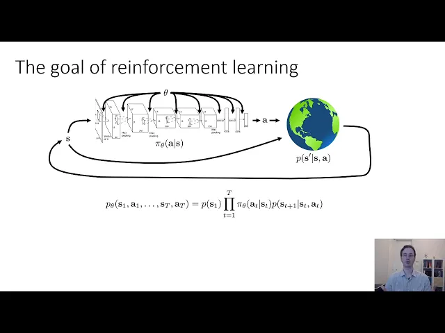
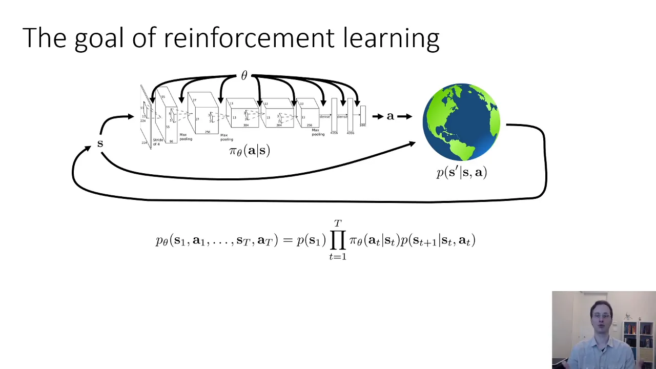
the policy directly and we'll see later on how there are some other methods that might represent the policy implicitly but for now we'll be explicitly learning pi theta a given s we'll come back to the partial observed case later for now let's just say that our policy is conditioned on s and theta corresponds to the parameters of the policy so if the policy is a deep neural net then theta denotes the parameters of that deep neural net the state goes into the policy the action comes out and then the state and action go into the

transition probability basically the physics that govern the world which produces the next state right so that's the process that we are controlling now in this process we can write down a probability distribution over trajectories so trajectories are sequences of states and actions s1a1 s2a2 etc etc until you get to state for now we will assume that our control problem is finite horizon which means that the decision making task lasts for a fixed number of time steps capital t and then ends we will extend this to the infinite horizon setting shortly but for now we'll write

down the finite horizon version because it's quite a bit easier to uh to start with so if we write down the joint distribution of our states and actions and here i'm putting the subscript theta on this joint distribution to indicate that it depends on the policy pi theta we can factorize it by using the chain rule in terms of probability distributions that we've already defined so we have an initial state distribution p of s1 i sort of brush this under the rug when i define the markov chain the mdp and the palmdp but all these

also have an initial state distribution p of s1 and then we have a product over all time steps of the probability of an action a t given s t and the probability of the transition to the next time step s t plus 1 given s d a t now i said this is derived from the chain rule of probability but of course in the chain rule of probability you need to condition on all past variables but here we are exploiting the markov property to drop the dependence on st minus 1 st minus 2 etc etc

because we know that st plus 1 is conditionally independent of st minus 1 given st so this is how we can define the tree distribution and for notational brevity i will sometimes write p of tau to denote p of s1 through sdat so tau is just a shorthand for trajectory and all it means is a sequence of states and actions okay so having defined the trajectory distribution we can actually define an objective for reinforcement learning and we can define that objective as an expected value under the trajectory distribution so the goal in reinforcement learning is

to find the parameters theta that define our policy so as to maximize the expected value of the sum of rewards over the trajectory so we would like a policy that produces trajectories that have the highest possible rewards in expectation and the expectation of course accounts for the uh stochasticity of the policy the transition probabilities and the initial state distribution so this is the definition of the reinforced learning objective that we're going to work with there are of course a few variants on this and we'll derive them over the course of the next few lectures this

is the most basic version so at this point i would like all of you to pause and look carefully at the subjective and really make sure that you understand what this means that you understand what it means to have a sum of rewards what it means to take their expectation under a trajectory distribution what a trajectory distribution is and how it is influenced by our choice of policy parameters theta which in turn influence the policy pi theta because if this part is unclear then what follows in the remainder of this lecture will be quite hard

to follow so please take a moment to think about this and if you have any questions about the trajectory distribution please be sure to write a comment on the video all right let's proceed so one of the things that we might notice about this factorization of the structure distribution is that it actually although it's a it's defined in terms of the objects that we had in the markov decision process it can also be interpreted as a markov chain and to interpret this as a markov chain we need to define a kind of augmented state space

so our original state space is s but we also have these actions and the actions make this a markov decision process but we know that the action depends on the state based on the policy so pi theta a t given s t allows us to get a distribution of our actions conditioned on states so we can do is we can group the state in action together into a kind of augmented state and now the augmented states actually form a markov chain so p of s t plus one comma a t plus one given s t

comma a t the transition operator in this augmented markov chain is simply the product of the transition operator in the mdp and the policy so this can allow us to define the objective in a slightly different way that will be convenient to use in some of our later derivations so so far i've defined the objective as an expected value under the trajectory distribution of the sum of rewards uh but remember that our distribution actually follows a markov chain with this augmented space and this uh transition operator is the product of the mdp transitions and the

policy so we could also write the objective by linearity of expectation as the sum over time of the expected values under the state actual marginal in this markov chain of the reward of that time step so this is just using linearity of expectation to take the sum out of the expectation so that you have a sum over t of the expectation over tau of r s d a t and then since the thing inside the expectation not only depends on state we can marginalize all the other variables out and we are left with a sum

over the expectation under p theta s t comma a t of r s t a t now this might seem like kind of a useless little mathematical uh you know kind of rewriting of the original objective but it turns out to be quite useful if we want to extend this to the infinite horizon case so this marginal p theta s t given a t in a finite time markov chain can be obtained just by marginalizing out all the other time steps but we can also use this objective to get the infinite horizon case so what

if t equals infinity well okay the first thing that happens if t equals infinity is uh your objective might become ill-defined for example if your uh reward your reward is always positive then you have a sum of an infinite number of positive numbers which is going to be infinity so we need some way to make the objective finite and there are a few ways of doing this uh one way of doing is well which i'll use now for convenience but is actually not the most common way is to use uh what's called the um the

average reward formulation so you basically take this sum of expected rewards and you divide it by capital t so basically the average reward overall time steps uh dividing by capital capital t is a constant so in general uh this doesn't change uh the maximum but then you can take t to infinity and get a well-defined quantity later on we'll learn about something called discounts which is another way to get a finite number for the infinite horizon case but uh so so making this finite is pretty easy but let's talk about uh how we can actually

define an infinite horizon objective so we have our markov chain from before and our augmented markov chain has this transition operator so that means that we can write the vector st plus one comma a t plus one as some linear operator t applied to st comma a t and this is the state action transition operator and more generally we can skip k time steps ahead and we can say that s t plus k a t plus k is equal to t to the power k times s d t so one question we could ask is

does the state action marginal p of s t comma a t converge to a stationary distribution basically converge to a single distribution as little k goes to infinity if this is true that means that we should be able to write the stationary distribution mu as being equal to t times mu and under a few technical assumptions namely ergodicity and the chain being aperiodic we can actually show the stationary distribution exists intuitively being a periodic simply means exactly what it sounds like that the markov chain is not periodic and being ergotic means that roughly speaking every

state can be reached from every other state with non-zero probability the ergotic assumption is important because it prevents a situation where uh if you start in one part of the mdp you might never reach another one so if you if this if this is true if starting in one part may result in you never reaching another part then where you start always matters and the stationary distribution doesn't exist but if this is not the case if there's even a slight chance of getting to any state from any other state eventually then you will have a

stationary distribution provided as a periodic so the station distribution must obey this equation mu equals t times mu because otherwise it's not a stationary distribution so stationary means it's the same before and after the transition and if it's the same before and after the transition then applying t enough times will eventually allow you to reach it you can solve for the station distribution uh simply by rearranging this equation to see that it is equal to tau tau minus i times uh so they can be written as tau minus i times mu equals 0. and remember

that mu is a distribution so it's a vector of numbers that are all positive and sum to 1. so one way you can find mu is by finding the eigenvector with eigenvalue one for the matrix defined by t so mu is eigenvector of t with eigenvalue one and it always exists under the ergodicity and aperiodicity assumptions so if we know that if we run this markov chain forward enough times eventually it'll settle into mu that means that as t goes to infinity this sum over the expectations of the marginals becomes dominated by the stationary distribution

terms so you have some finite number of terms initially that are not in the stationary distribution mu1 mu2 mu3 etc then you have infinitely many terms that are very very close to the stationary distribution which means that once you put in the average reward case so you're going to find put a 1 over t and then take the limit as t goes to infinity the limit is basically going to be the expected value of the reward under the stationary distribution and that allows us to define an objective for reinforcement learning in the infinite horizon case

as t goes to infinity okay this is perhaps a lot to take in so this would be a good place to pause think about the derivation on this slide and if something is unclear or you have any questions please be sure to write them in the comments all right now one uh last bit that i want to describe in this section which is very important for understanding the basic principle behind a lot of reinforcement learning methods is that reinforcement learning is really about optimizing expectations so although we talk about reinforcement learning in terms of choosing

actions that lead to high rewards we're always really concerned about expected values of rewards and the interesting thing about expected values is that expected values can be continuous in the parameters of the corresponding distributions even when the function that we're taking the expectation of is itself highly discontinuous and this is a really important fact for understanding why reinforced learning algorithms can use smooth optimization methods like gradient descent to optimize objectives that are seemingly non-differentiable like binary rewards for winning or losing a game let me explain this with a little toy example let's imagine that you're

driving down a mountain road and your reward is plus one if you stay on the road and zero if you fall or negative one if you fall off the road so the reward function here appears to be discontinuous there is a discontinuity between staying on the road and falling off the road and if you try to optimize the reward function with respect to for example the position of the car that optimization problem can't really be solved with gradient based methods because the reward is not a continuous or much less a differentiable function of the car's

position however if you have a uh probability distribution over some action let's let's say that abstractly that you just get to choose like fall or don't fall so you have a binary action the other fall you don't fall and it's a bernoulli random variable with parameter theta so with probability theta you fall off with probability one minus theta you don't fall off now the interesting thing is that the expected value of the reward with respect to pi theta is actually smooth in theta because you have a probability of theta falling off which has a reward

of minus one and a probability of one minus theta staying on the road so the reward is one minus theta uh plus uh one minus theta minus theta and that's perfectly smooth and perfectly differentiable in theta so this is this is a very important property that will come up again and again and that really explains why reinforcement algorithms can optimize seemingly non-smooth and even sparse reward functions which is that expected values of non-smooth and non-differentiable functions under differentiable and smooth probability distributions are themselves smooth and differentiable okay let's pause there