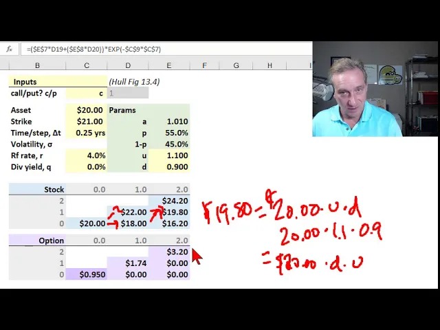
my previous video introduced the binomial option pricing model but in that version I just arbitrarily made up the values for U and D U and D represent respectively the magnitude of the up-and-down jump in the model so they inform the stock price tree here how much does this $20 jump up or down in the binomial now I'd like to just articulate the intuition behind a common step that we take when we use maybe the most popular version of the binomial option pricing model that's this version it's called the Cox Ross Rubinstein and in this version now we have a volatility input assumption just like we do with the black Scholes and we let that volatility inform for us the U and the D or it's John hull says it we match volatility with U and D so we don't need to make it up why does that work what's the intuition that's what I'd like to show you now so my baseline assumption here is a two step binomial option pricing model based on the same assumptions that are found in John hole's textbook that's the tenth edition this is assigned to a farm candidates and you can find that in figure thirteen point four so that's in Chapter thirteen although my presentation differs in terms of the stock price tree that we build out and the option value node I'm using the lower triangle format because this is only a two step binomial that's unrealistic when we get to more steps this triangle format ends up being I think much more convenient so we break out the stock prices up here and the option value notes here and this process is leading us to the solution which is found right here in darker purple the price of this six-month option for a two-step binomial you can see is 95 cents that's based on assumptions here you can download the spreadsheet which includes the ability to toggle this between a call or a put small C I remind you denotes European not a american-style call option we have an asset of $20 so that's s sub-zero that's the price at the time of purchase of the option in the strike price here is $21 so this call is going to be slightly out of the money key input here is the time per step or per interval as usual our input assumptions are always in per anum so the time step you can see here is 0. 25 years which of course is 3 months and that refers not to the overall life armature the option but rather just the time per each step this is a 2 step up binomial option pricing model and so that's two steps times three months per step it's six months to maturity on the option is this assumption so I'm not going to use a volatility input that's gonna be on the next sheet because here I'm just setting up the baseline to show you the difference our risk-free rate is 4% I'm assuming a dividend yield of 0% and then we have the solved for parameters that are the key ingredients in this binomial option pricing model so in green they're solve for an in yellow I have the two inputs that we manually specify same as I did in the last video but you'll notice the P and 1 minus P are solved for and I mentioned in the introduction video that these are solved for that important component here of the binomial option pricing model which is risk neutral valuation so the risk neutral valuation allows us to solve for the probability of an up jump in this binomial model which is given by e raised to the R minus Q risk-free rate minus the dividend that quantity is the a right there so we didn't need to explicate the a but sometimes this makes it a little easier to explicate the a that's just the a right there and we subtract D magnitude of a down jump divide that quantity by the difference between U and D so P is solved for us per formula and why do we have that formula well it's an it's necessarily true in the risk-neutral valuation framework without basic ideas were allowed to solve for this in the risk-neutral world and transfer the truth of that over to the rural world so we get the probability of an up move and therefore 1 minus P is the probability of a down move and you can see those probabilities are respectively 55 and 45% what I needed to provide as I did in the last video introducing is values for up and down and here I follow John hull assuming that if the stock jumps up it'll go up 10% if it goes down it'll go down 10% so we have multipliers of 1. 1 and 0.
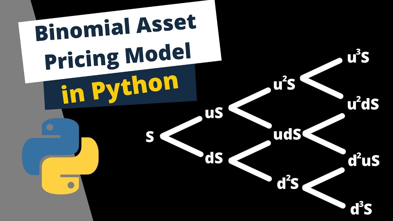
9 and you'll notice that's there's a symmetry there in the plus 10 or minus 10% right so plus or minus 10% these are manual assumptions under this baseline approach that I'm going to replace in the next sheet but we needed the up or down of course to specify the stock price tree that's that first major step in the binomial here where we start with the initial asset price S sub 0 right and that in the binomial by definition that price at each step is going to either go up or it's going to go down we're in this triangle format down is just to go down is to stay on the same row so you can see the $20 either goes up by 10 percent to 22 or it goes down by 10 percent to 18 and similarly the 22 either goes up to 24 point 2 or goes down to 19 point eight and I do have here I've included in this exhibit this worksheet these this row and column which help with the notation I like this tree notation I got from Bruce Tuckman actually and that is to say this $19. 80 right here well that is we could refer to that as the node at date comma state is the way that works so date refers to counting over the number of columns starting at 20 if we go one two where two dates over like that and then we start at the bottom with the zero width so the 16 20 is state zero the 19. 8 is state so the $19.
80 is the value at the node two comma one if we want a reference but that Nate 1980 is equal to the $20 the initial stock price assumption multiplied by an upjumped multiplied by a down jump which of course is $20 here multiplied by 1 point 1 and then multiplied by 0. 9 right so we could go up and then down and we get there and as I mentioned the previous video we're keeping things simple with a recombining tree so this $19 and 80 you get to that same value if the $20 were to go down then up if we switch them around right so $20 could drop to 18 but then go back up to the same 1980 so that if we have two steps were necessarily by definition going to end up with three terminal values and so that first major step is a simulation forward and so the point of that is to retrieve these three terminal values that's at the end of six months right two steps each step is three months so six months to maturity of the option so really this terminal this point in time is determined as a contractual feature or specification of the option contract happens to be six months here it could be one year could be three months so we take the terminal values and then perform the second step here which was technically we call that backward induction you might recall and in the backward induction we're really just implying a fundamental principle of Finance which is we're computing the expected discounted value at each node so if I take this one set this dollar 74 which happens to be at the node 1 1 right date one step state one step up node 1 1 has a value of dollar 74 how did I get that it's just X affected discounted value there's a 55% probability of a of a forward option value of 320 based on the intrinsic value at terminal at termination or maturity or there's a plus a 45 percent probability of a 0 so 55 percent multiplied by three dollars and twenty plus forty five percent multiplied by zero gives us that expected value six months forward that we then discount at the risk-free rate I think I covered that in a little more detail in the previous video our introductive devine introduced the binomial don't want to go not in there right now but just to remind that we're getting this node with expected discounted values same here the expected this kind of value of two zeroes is just zero that one's easy and we did we get expected this kind of value one more step as part of the backward induction gets us to the option price of ninety five cents which by definition here then is a present value of course the option pricing model is computing for us a present value however now point of this video is really that we had to go find an up internet or go make up an up-or-down value of play in this case plus or minus ten percent and if that feels arbitrary I think it's safe to say that it is arbitrary why not twenty percent went up 15 percent well that's the point of matching the volatility to the up and down parameters and I'll also note that you'll notice this symmetric as we increase the number of steps in the binomial we are also implicitly assuming that these arithmetic returns are normally distributed like to keep that in mind this assumption here implicitly is that arithmetic returns are normally distributed but now what I do on the next sheet also in the downloadable works if you want take a closer look is now I'm going to use the volatility parameter so this is what Hall calls matching volatility with the up or down and if I happen to use a moment I've just changed out 30% let's say an put a 30% the idea here is that now I don't manually need to make up or arbitrarily my upper down inputs and from an exam perspective most the time you'll be given the volatility and you solve for the und so that's how that works now these aren't yellow anymore they are solved for and the solution is super simple the up jump is simply arrays - and what all we have in the exponent is the periodic volatility it's that simple we're taking an exponential of the periodic volatility and the periodic volatility is the 30% that we're given right so I'm just gonna say 0. 3 or here I'm just going to represent symbolically the up is e raised to our volatility which is in this case a 30% however the 30% again is a per annum and each of but each of these steps are only three months so we scale that to the correct periodic Villa volatility which is to say what is the three-month volatility well it's the 30% multiplied by the square root of time so for frm candidates that should be familiar because we're employing the square root rule what we have in the exponent here is simply the 3-month volatility that were that is just translating the assumption that we're given that square root role of course assumes iid I'll plug that up just up here the independent and identically distributed that's the implicit assumption in that square root rule so we are using that that's the you it's that simple D is just 1 divided by u or if we want to just if we want to really explicate it it's then in the exponent we just have the negative of volatility scaled by the square root of time right standard deviation skills go at a time because variance scales with time but it's easier just to say 1 divided by u so the U and the D match the volatility or we take the volatility input assumption to infer for us what the correct U and D are and now why does that work well John Hall actually shows the Dera fication the derivation of that but I just want to show you the intuition and the intuition is simply that we are solving for the U and the D that gives us a binomial random variable with this volatility it's that straightforward it's really I'm really just restating the fundamental assumption in the first place we want to match up and down to the volatility why do these values work they work because these are the up and down values that give us the standard deviation of a binomial variable equal to approximately 30% it's easy to forget well maybe not that we have a binomial tree and what that means is we really have at each node here a binomial random variable so all I've done here is just transfer these over the one point one six and point eight eight point six eight point eight six one that is solved for if I just subtract one these are returns right now when these revive rise values the U of 1 point 1 6 2 is a multiplier so it's telling us that if we jump up we're jumping up by sixteen point two percent and then here's the probability P forty nine point six and here is the one minus the probability fifty point four so here I'm just restating the same values but now we have return and probability and then the key insight is simply just to remember that this is a binomial variable I sometimes like to think it's a Bernoulli variable because it's just up or down but technically a Bernoulli requires values of and zero and we actually we actually have an up returning it down return so these are not 1 and 0 so to me it's sort of like a Bernoulli but it's sent as the simplest possible binomial and what is the variance of a random variable well our most important or a most common or useful variance formula if I'm going to take the variance that Sigma squared of a random variable are our most useful property of variance is that it's the expected value of R squared minus the expected value of our quantity squared right I hope that's familiar and you could put an X in there and might make it a little more familiar for using X but that is a key and fundamental property of the variance so all that I've done here is apply that formula for the variance of a binomial and I to get it right here so I have here the expected value of r-squared you can see is simply if I take the return and square it and multiply by the probability but let me do that again return and square it multiplied by the probability and you can see if I do that for the down and then if I sum those I get zero point zero two three so that's the expected r-squared and then here this is even more simple here I just have the return times the probability so that this so that if I sum those I get the expected return and then I'm going to square that quantity so you can see here point zero two three as my expected the expectation of return squared and point zero zero zero one zero is the expected return as a quantity square so that if I take the difference of those I am simply computing the variance of this binomial random variable and this variance is point zero two two seven such that if I take the square root of it I get the standard deviation or the periodic volatility which is fifteen point one percent and if I compare that to my input assumption I I just take the 30 percent and again that's per annum so I want to scale that to the periodic or three-month volatility by multiplying by the square root of 0.
25 so that when I input assumption my 30 percent per annum input assumption is the same as a three month input assumption of fifteen percent volatility so I'm comparing it to the assumption that I was given and you can see that's the point matching the volatility with the up or down to do that is to find the upper down values that when used in the binomial random variable which each of these nodes is dynamically model we get a variance and therefore a standard deviation and therefore a volatility equal to the volatility input assumption in this case it's about 15 and you'll notice it's not exactly the same but if I take the if I put this down at 20% I think where I first found it you can see they're gonna they're gonna again approximate each other but it's not going to be exact and if I take that out and that's because Hall in a derivation the math this is a mathematical derivation to make these match however to keep the derivation simple he is allowed to ignore some higher power terms in the nor a math that they just shave a little off the difference so we end up with a little bit of approximation so I think it's fair to say this will always be just slightly different than the than the actual input value but we now don't need to arbitrarily guess what the up or down is we're using the volatility input assumption to open form it and the final thing I would just say about that is that recall in my baseline where we used our oath medic we were symmetrical with a plus up plus down well I said that implicitly that's arithmetic returns normally distributed here we're not symmetrical right that's because down is not equal to negative up or one minus up it's one month it's one divided by you it's the reciprocal of the up so these aren't symmetrical and you can see that even visually here this is 10.