Mixed Precision Training | Explanation and PyTorch Implementation from Scratch

The idea of using GPUs for neural network training dates back as early as 2004. GPUs can launch thousands of lightweight threads, each handling a small independent computation in parallel. And that's exactly what neural network training needs.

Think about matrix multiplication. One of the most compute operations in neural networks. Every element in the output matrix can be computed independently.

So instead of calculating them one by one sequentially, GPUs can process thousands of them at once, giving a massive speed up over CPUs. But as the field has evolved and our models have grown larger and more complex, the compute demand has exploded almost exponentially. Every new generation of neural network brings about billion more parameters and with that the cost to train them has been doubling nearly every year.

Whether we use high-end GPUs that train faster but cost a fortune or cheaper ones that train slower, the total compute cost continuously keeps on rising. That's why in this and in some of the future videos, we'll focus on techniques that make training more efficient, letting us train larger models with fewer resources. And the first technique, the focus of this video is mixed precision training.

Before we talk about mixed precision training, we actually first need to understand what precision really means. And to do that, let's see how floatingoint numbers are stored in our machines. Let's take the number pi as our example.

In decimal form, it looks like this 3. 1415 and a lot of numbers after that. But when stored in our machines, it's represented using a specific floating point format.

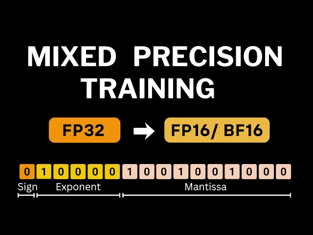
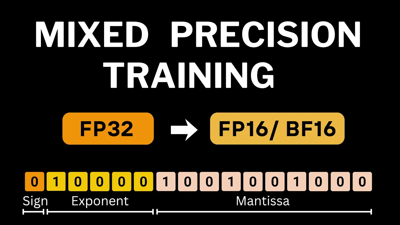
The most common one used for deep learning is float 32 also known as single precision. A float 32 number is made up of 32 bits in total. One bit for sign, zero means positive and one means negative.

Eight bits for the exponent and 23 bits for the mantisa also called the significant. All floatingoint numbers follow the same scientific notation form that is a one followed by radics point. Then whatever is in mantisa this 1 point mantisa is then multiplied with 2 raised to the power of exponent and we have the sign bit taking care of whether it's a negative or positive number.

Let's decode the bit pattern of pi to see this. The sign bit is zero. So it's a positive number.

The exponent bits are one and then a bunch of zeros. To convert this binary form into decimal form, we use the same steps as integers. Assign powers of two to each digit starting from the right beginning with power zero.

Then multiply each binary digit by its corresponding power of two and sum them all together. This comes out to be 128, which could and in fact should seem weird. After all, it's too high for our number pi.

But this is not the true exponent value. The true exponent value is 128 minus 127 where the magic number 127 is called the exponent bias for float 32. The reason this bias exists is so that we can represent negative exponent values as well as positive.

So if you had to represent a number which has true exponent as say minus 126 in memory its exponent will be represented as -26 + 127 which is 1. So rather than just representing 0 to 255 positive exponent values we can represent exponent values ranging from -27 to 128. In reality, some of these exponent values like minus 127 and 128 are reserved for special numbers like 0 and infinity.

So our true exponent range for float 32 is from -26 to 127. Using the exponent bias of 127, the exponent value for pi comes out to be 1. The mantisa bits represent the fractional part.

Starting from the first bit after the radics point, each bit contributes a value of 2 raised to the power of its negative position. So the first bit contributes 2 ^ -1, the next one 2 ^ -2 and so on. We then add one which is the implicit leading bit to the fractional value.

This leading one is always implicit and since it's always going to be there, we never actually store it allowing us one extra bit for representing the fractional part of the number. So our float 32 number becomes 1. 57 something something * 2 raised to ^ of 1 which is very close to the value of pi.

Now that we know what exponent and mantisa are, this is a perfect time to talk about how they decide our representational capability. With 8 bits for the exponent, float 32 can represent exponents from 0 to 255. After accounting for bias, the true range is -27 to 128.

And as I had mentioned earlier, the highest and smallest value is reserved for special numbers. So the actual range of exponent values was minus 126 to 127. The largest value that can be represented by the 23 bits of mantisa is this.

And the smallest of course would be zero when all mantisa bits are zeros. Which means the largest number that we can represent in float 32 format is approximately 3. 4 * 10 raised to the power of 38.

And the smallest positive number is 1. 17 * 10 raised ^ of minus 38 giving float 32 a huge representational range. Actually numbers smaller than this can also be represented in float 32.

But those are stored with an exponent of all zeros and a nonzero mantisa. These numbers are called denormalized or subnormal numbers. In such cases, the implicit leading bit, the hidden one, is actually replaced by zero.

For subnormals, the effective exponent is taken to be -26. So, the smallest positive subnormal number in float 32 becomes 2 ^ of -23 * 2 ^ of -26, which gives us 2 ^ of -49. By the way, if exponent is all zero and mantisa is also all zeros, that represents the number zero.

Coming back to representational capability, the number of bits in the exponent decides a range of representable numbers. Larger number of exponent bits means larger range of values can be represented. Mantisa on the other hand decides how accurately we are representing that number or more specifically how finely we can represent fractional values.

More number of bits in mantisa means we have more accuracy. This is what's meant by precision as more bits in mantisa means we can precisely represent our number. The largest and smallest positive numbers one can also get if you inspect the representation details of float 32 in your deep learning framework.

So all this that we have been talking about was for float 32. Now with this understanding let's look at some of the other floating point representations. In this video we are going to be talking about float 16 and brain floatingoint format also known as Bflat 16.

For float 16, Mantisa only has 10 bits and the exponent is also reduced to just five bits. Because of the reduction in exponent bits, the range of values that can be represented by float 16 is significantly reduced, especially compared to the range that we were working in float 32. Smallest normalized positive number for float 16 is 2 raised ^ of -14 and the smallest denormalized positive number for float 16 comes out to be 2 raised to ^ of -4.

To see this you can do a similar calculation that we did for float 32. Values smaller than this would underflow to zero. Do keep note of these two numbers as we'll use them in our discussions in mixed precision training.

Values larger than this will cause overflow in float 16 and end up being represented as infinity. V float 16 further reduces the number of bits for mantisa which is just 7. However, the bits for exponent remains the same as float 32 making its range similar to that of float 32.

Since the bits for Mantisa keep getting reduced from float 32 to float 16 and then further reduced in Bflat 16. The precision also keeps on reducing. But there are a couple of advantages of Bflat 16.

First is that we get the same range as float 32. So numerically it's more stable and less prone to underflow. The second advantage is that converting float 32 to B float 16 is very easy.

Just round off 23 bits of mantisa to 7 bits. And on the other hand, float 32 to float 16 conversion is not easy since the exponent size also differs. The number pi in float 16 as well as b float 16 ends up being represented as 3.

140625 which shows what we lose in precision when we move away from float 32. The difference in precision is quantified using epsilon. the smallest number that when added to one gives the result greater than one.

Each format has its own epsilon value. Smaller epsilon means higher precision. A good way to look at these three representations is to think in terms of a measuring tool which has a certain length and tick marks indicating how precise value that tool allows to measure.

Larger length means you can measure objects of larger length and finer tick marks means you can measure length more precisely. For float 32, we get the maximum range and very fine tick marks. Bloat 16 has the capability to measure the same length, but the tick marks are coarser.

For float 16, we have a much smaller length than the other two, but the pick marks is slightly finer than B float 16, but still coarser than float 32. Now that we understand precision and what we lose upon moving to lower precision that is numerical accuracy, let's look at why lower precision can actually be a good thing for training deep learning models. The first advantage is memory savings.

When we train a model, all of its parameters are moved to GPU. Then during backward pass, gradients are computed for every parameter. Then we have optimizer states.

And for optimizers like Adam, there are two additional tensors maintained for each parameter. The first moment estimate and the second moment estimate. And of course during the forward pass, intermediate activations are generated.

Activations in particular grow rapidly with larger batch sizes. And since GPU memory is finite, this usually becomes the main bottleneck that limits how big a batch we can use. Now all of these tensors are typically stored in float 32 format which uses 32 bits per value.

If we switch to a lower precision format say float 16 each value now uses just 16 bits. That's half the memory per tensor element. This means we can now either fit larger batch sizes into the same GPU memory and larger batch sizes often lead to smoother gradient and faster convergence or we could fit larger models that previously would have caused out of memory errors.

The next advantage is speed. Since each value now takes up half as many bits, data transfers between GPU memory and compute cores happen faster. This reduces memory bandwidth bottlenecks.

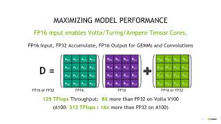
But the biggest speed up comes from hardware level optimizations. Modern Nvidia GPUs come with tensor cores, specialized processing units designed to perform matrix multiplications using lower precision data types like FP16 or BF-16. The operation of computing products of matrix A and B to produce output C is at the heart of nearly all deep learning models.

Tensor cores perform a whole block of matrix multiply accumulate operations in a single clock cycle compared to CUDA cores which would take multiple clock cycles to perform the same work and that's what provides the speed up. So when training leverages this dedicated low precision hardware it becomes faster than standard FP32 training. These were the main reasons to prefer lower precision during training.

In the next section we'll implement mixed precision training from scratch. We'll start with a simple training script in FP32 and then progressively convert it to FP16. We'll focus on FP16 because even older GPUs support FP16 acceleration.

By making the changes manually, we'll see every piece of the puzzle, what needs to change and why, which would make the concept much clearer. Finally, we'll see how to use PyTor's automatic mixed precision, which abstracts most of these details away and lets you move from single precision to mixed precision training with just few lines of code. For implementation, we'll be following along this paper.

We'll kick off things by training a simple image classifier on the MNEST data set using the default FP32 format. At the top of our training script, we have transformations to convert MNEST images to 3 + 224 cross 224. Then we have our training and test data loader.

Our model is VG16 and we use torch visions VG16 module itself and simply specify the desired number of classes as argument. The loss is standard cross entropy and we use SGD as the optimizer. This is the method which trains for one epoch and inside the loop we'll get the image feed it to our model compute loss and gradients and update parameters.

We also have a test method that computes classification accuracy on the test set. The whole script is intentionally simple about 70 lines and after training for five epochs we get a loss curve that falls nicely. We not trying to get the best possible model here.

We just want a baseline so we can observe the effect of switching to lower precision. Before we change anything in this FP32 training code, let's break down how much memory different parts of the training use. Model parameters take roughly about 500 MB and so do the gradients.

With a batch size of 64, activations in the forward pass take about 3. 6GB. And with Adam as the optimizer, optimizer states take twice the parameter memory because Adam keeps both the first and second moment estimates for every parameter.

That gives a total memory consumption of around 6GB for VG16. Now let's try training in lower precision FP16. For this we can simply cast the model parameters and inputs to FP16.

In code, that means first casting all FP32 parameters to FP16 by simply doing model. And then we do the same for our input image tensor, casting it to FP16. This two-line change causes our parameters, activations, and gradients all to be stored in half precision.

Let's see the memory breakdown. Now these were our FP32 numbers and on the right we'll have respective values for FP16 because FP16 values are 16 bits instead of 32. Each tensor now uses half the bytes.

So in our observed numbers the total memory drops roughly to 3 GB. This is great. I mean now we can use much larger batch sizes or even bigger models if we need to.

And on top of it, we also get a speed benefit as training time also reduces by about 15%. But sadly, when training using this casting approach, the FP16 loss doesn't decrease as compared to FP32 training. The culprit here is FP16 arithmetic and its limited precision and range.

To understand why this happens, let's start with the weight update equation. The change in a weight value is simply the learning rate times the gradient of the loss with respect to that weight parameter. For example, a particular parameter in our VG model has a value of 0575 and the gradient for it is 1 eus 3.

Our learning rate is also 1 eus 3. So the change is close to 1 - 6. But when we try to apply this update in float 16, the weight value doesn't change at all.

In fact, forget about 1 - 6. Even adding 1 - 4 to 1 in float 16 doesn't produce a value different than 1. To really understand this, let's look at what's happening at the bit level.

Float 16 has one sign bit, five exponent bits, and 10 bits for the mantisa, the part that controls precision. For the number one, the stored exponent bits are 0 and four 1's which corresponds to 15 in decimal system and the mantisa bits are all zeros. Let's just check whether this bit sequence indeed comes out to be 1 or not.

We have the implicit leading bit as one, mantisa as zero and the true exponent is 15 minus bias where the bias is 15 for float 16. So 15 - 15 equals 0. So yes, this sequence of bits indeed represents one 1 eus 4 is this sequence of bits and you can verify that this evaluates to 1.

6386 * 2 raised to ^ of 1 - bias which means -4 which is very close to 1 - 4. So let's add 1 and 1 e - 4 together. These are their binary representations.

And the first thing we do to add these two binary numbers is aligning their exponents. That is done by aligning smaller exponent to the larger one by shifting its mantisa bits to the right. So for 2 raised ^ 1 minus bias, we'll have to increase its exponent by 14 to get to 2 raised to ^ of 15 minus bias.

Which means the radics point will shift 14 places to the left. Or you can say that the mantisa bits will shift 14 places to the right. Once we do that and add the two, those shifted bits fall well beyond the 10 bit mantisa precision of FP16.

So their contribution is lost. As a result, the sum remains one. The small addition of 1 - 4 has no effect.

In fact, earlier we looked at epsilon, the smallest number which when added to 1 leads to a number greater than 1. And for FP16, it was a number greater than 1 - 4. Which is why adding 1 to 1 - 4 is just 1.

Now connecting this to training, weight updates are often smaller than the smallest representable addition in FP16. Which means during FP16 training, the updates won't change the stored weight because the change happens outside the mantisa. And that is the problem.

But what's the solution? Well, what if we change just these two things? We initialize our W in FP32 rather than FP16 and then cast the final W to FP16.

Now, the initial FP32 weights do get updated properly. This is because when you add an FP16 value, the gradient to a FP32 value, the weight, the FP16 operant is automatically promoted to FP32 before the addition. This means the operation takes place in FP32 precision which has a 23-bit mantisa allowing those very small updates to actually affect the weight and then even when you cast the updated weights back to FP16 those tiny accumulated changes over many steps are now large enough to be representable even in FP16.

So the final FP16 weights indeed reflect the update. With this knowledge, we'll make some changes in our training script. Up till now our weights were only in FP16.

During forward pass we computed activations in FP16. Then after computing loss we back propagated and computed gradients also in FP16. These gradients were used to update FP16 weights.

But that we have seen can be problematic and might not lead to any change at all. The fix that we will use is to maintain an extra FP32 master copy of the parameters. So we already have our FP16 parameters for forward and backward pass and that is going to give us the memory and speed benefits but in addition we maintain a corresponding FP32 copy of every parameter after back propagation and computing FP16 gradients.

These gradients are copied to the FP32 parameter gradients. And now rather than updating FP16 weight, we use these FP32 gradients to update the FP32 master copy of parameters in single precision. Finally, the updated FP32 weights are copied back to FP16 model so that the next forward pass uses these updated FP16 weights.

Because the parameter update occurs in FP32, the small increments are represented correctly and so updates ultimately change weights even in FP16 precision. So let's see how this change is implemented in code. The first thing that we do is create a copy of parameters in FP32.

Our optimizer will actually be updating these FP32 parameters itself. So here rather than model. parameters, parameters.

We pass these. Then in our training loop, we do model. 0 in addition to optimizer.

0. This is because the optimizer is going to clear the gradient of FP32 parameters and model. 0D will ensure that gradients of the FP16 model parameters are cleared.

Since the model parameters are in FP16, after this loss dot backward, we have our FP16 gradients. Then we are going to copy these gradients onto the FP32 params copy that we had created earlier. This entire section does exactly that.

loops over the FP32 parameters which do not have gradients and FP16 model parameters which indeed have gradients and then copies the gradient from FP16 parameter to the FP32 one. The last part is updating the FP32 parameters and copying the updated values to FP16 model parameters and that is done via this block of code. Optimizer.

step step we'll update the FP32 parameters because that is how we initialized our optimizer and then in these lines we are just taking each updated FP32 parameter and copying the updated value into the FP16 model parameter. With this change the forward and backward pass still happens in FP16. So activations remain low memory and yet parameter updates happen accurately in FP32.

Now our training ends up with a similar loss plot as FP32. But doesn't this extra copy of parameters wipe out all the memory gains that we saw earlier? Well, not exactly.

Activations tend to dominate peak memory. So the extra memory for FP32 copy is usually acceptable and the memory consumption will still be lesser than that of FP32 training. For our case of VGG on MNEST data set, these changes alone are sufficient to ensure successful FP16 training.

But there are scenarios where we need two additional changes. First one that we'll talk about is loss scaling. Even with a FP32 master copy, you can still lose gradients as the gradients themselves can become zero when computed in FP16.

To analyze this, let's plot a histogram of the log of absolute gradient magnitudes during a random step in FP32 training. The smallest normalized FP16 number is 2 raised ^ minus14 and the smallest subnormal is 2 ^ minus4. Here as you can see most of the gradients are greater than that number.

But what if this was our gradient distribution? Now a large fraction of gradients would actually underflow to zero in FP16. And why is that?

Because FP16 cannot represent such small numbers since we only working with five exponent bits. Note that this is not really a problem for Bflat 16 because that has the same exponent range as FP32. So underflow is far less likely there.

But for FP16, this indeed could be a problem. And the solution is loss scaling. Prior to FP16 backward pass, we multiply the loss with a large scalar value S.

Then after backdrop, all the gradients will now be scaled by S. And the gradient distribution is going to shift towards the right. How far it shifts will depend on the value of S.

But using a large enough value, we can ensure that most of the gradients are in FP16 representable range. After backward pass, prior to actually updating the FP32 weights, we divide or unscale the gradients by S. That way, the final gradient values applied to the FP32 master parameters are exactly the same as they would have been without loss scaling.

This basically ensures that because of loss scaling, we don't need to change any hyperparameters in code. This just requires adding two lines of change. First we'll scale the loss prior to calling loss dot backward we'll use a fixed value of say 8192.

Then after copying the FP16 gradients to FP32 parameters we'll unscale the FP32 gradients by the same factor. Here I've used a fixed scale factor but in practice we use dynamic loss scaling where we start with a large scale value and monitor for any ends or infinities during training to adjust the scaling factor. We increase the scaling factor when it's safe and decrease it when instability occurs.

All the changes that we have made so far dealt with parameters and gradients. But there's one last piece that we need to handle for mixed precision training and that concerns with the numerical stability and accuracy of certain operations inside our neural network layers. Some operations involve large reductions like computing mean or variance.

It actually makes more sense to perform these in FP32 rather than FP16. This is because in FP16 the limited mantisa can lead to significant rounding errors when many small values are summed together. Also, the sum itself can easily exceed the maximum representable value in FP16 leading to overflow.

Similarly, operations like exponentials are also safer to perform in FP32 because they can produce very large or very small numbers which again would lead to overflow or underflow in FP16. To handle this automatically, deep learning frameworks implement per operation precision policies. Meaning some operations are done in FP16 if it's safe to do them in FP16 and the others in FP32 when using lower precision isn't safe enough.

So mixed precision training combines everything that we have implemented so far plus the operation level casting rules that preserve numerical stability and accuracy. But when using a framework's built-in mixed precision utilities like PyTor's AM, everything is handled by the framework and converting FP32 training script to mixed precision training script is often just a few extra lines of code. Let's see exactly what those changes are by converting our initial FP32 training script to one that uses PyTor's automatic mixed precision.

First, we are going to go back to our FP32 training code. So I'll simply delete all lines of code that I added to handle FP16 precision. This includes the FP32 master copy converting the model to half precision.

Our optimizer will now work on the original model parameters and we don't need to convert the input to half precision. Let's also remove all the code that we added in this loop. And we also don't need this model.

Okay, so this is our original FP32 training script. Using the PyTor's automatic mixed precision requires us to just add four lines of code. We first initialize an instance of grad scaler class.

This class takes care of scaling loss, unscaling gradients, and updating our parameters. Our forward call will be wrapped under this autocast context. Autocast chooses the best data type for each operation for the code block under it.

Wherever it's possible to run that operation in FP16 without loss of accuracy, AutoCast will use FP16. But wherever it's necessary for that operation to run in FP32 like batchnom exponentials autocast will ensure that those run in FP32 rather than loss dot backward here we'll first scale the loss and then run backward pass that rather than optimizer. step step we'll have scalar first unscale the gradients and then update the parameters which is what this line does and finally we'll call scalar dot upupdate which will update the loss scale factor depending on whether there were any infinity or any n gradients in previous steps autocast chooses per operation precision and gradcaler handles scaling unscaling and dynamic scaling adjustments that's actually all the change that you need for mixed precision training in PyTorch.

As you can see, the actual code change for mixed precision training was really small. But I wanted to go through step by step and show how one can actually implement mixed precision training themselves without using the framework utilities. Hopefully that made the mechanics of mixed precision clearer and you understood why exactly we needed FP32 weights or loss scaling and generally what are we losing and gaining when we are moving to lower precision training.

In the future videos, we'll also look into quantization and other similar topics. So, see you then. Thank you so much for watching this one.