[Music] hello everyone welcome to this lecture in the build large language models from scratch series we have been covering attention and the attention mechanism in a lot of detail for the past two or three lectures the lectures were long they were more than 1 hour each but I think it's extremely important for you to understand the attention mechanism and Uh that's why I'm devoting so much time to these set of lectures just to give you a quick recap of what all we have covered so far in this in the first lecture on attention we started
with a simplified self attention mechanism without trainable weights in the previous lecture we added trainable weights and we discussed the self attention mechanism with trainable weights here we also looked at the concept of key query and values which We'll revise just in a moment and then today our main aim is to learn about something which is called as causal attention after learning about causal attention in the next lecture we'll move to multi-head attention which is the actual attention mechanism which is used in GPT and other modern large language models I believe this sequential flow is
extremely important because if you start understanding multi-head attention directly you will not understand the Basics you will not understand the nuts and bolts of what exactly is attention how did we we get to multihead attention so let's get started with today's lecture on causal attention Okay first let us revise everything we know about self attention what we have learned in the previous lectures so the example which we have started looking is this one sentence which is your journey starts with one step so you'll see that there are six Words in this sentence the first step
of any um data processing pipeline for a large language model is to convert these words into tokens to convert these tokens into token IDs and to convert the token IDs into Vector embeddings so here you can see that for each token we have threedimensional Vector embeddings so for the token y we have a three-dimensional Vector embedding for the token Journey we have a three-dimensional Vector embedding and For the token step we have a three-dimensional Vector embedding remember generally one word is not equal to to one token because uh GPT and other modern llms use a
bite pair encoder which are sub tokenizers but for the purposes of this lecture I'm going to use word and token interchangeably okay so the first step is to convert all of the tokens into Vector embeddings I'm choosing a three-dimensional Vector embedding here Just for the sake of demonstration remember that in models like GPT it's common to have Vector dimensions of 500,000 or even more Ive just plotted these vectors and how they look like over here in the three-dimensional space these are the input embeddings the goal of any attention mechanism is to take these input embeddings
for every vector and convert them into context embeddings or context vectors for every token now what's the difference between uh input Embedding and context embedding or a context Vector so let's say if you look at the journey this is an input embedding for Journey this green Vector which you see over here which contains which encodes some semantic meaning about Journey but it does not carry any information about how the other words in the sentence such as your step with one how all these words relate to Journey how much attention should you Pay to each of
these words when you are looking at Journey the embedding vector or the input Vector for Journey contains no such information whereas the context Vector contains this information the context Vector not only contains semantic meaning about Journey but it also encodes meaning about how Journey relates with all these other words so that's the main aim of the attention mechanism to get context vectors for each of our input embedding vectors why Do we need context vectors because it makes the task of the next word predictions much more better much more reliable because now we are encoding information
of how much attention needs to be paid at different words in a sequence of sentences so that's the whole aim of attention mechanisms as we saw in the previous lecture the first step is to multiply the inputs with the query Matrix the key Matrix and the value Matrix when you multi when you do this multiplication you get the query query Matrix so there's a difference so this WQ w k and WV are weight matrices so these are the trainable weight Matrix this is the trainable query Matrix this is the trainable key Matrix and this is
the trainable value Matrix you multiply the inputs Matrix with these trainable weight matrices and then you get the final queries Matrix the keys Matrix and the values Matrix that's the first step now remember that this WQ w k and WV these training weight matrices are not fixed their parameters need to be trained based on input data and this training is a part of the llm currently when we are learning attention mechanisms we are not learning about this training procedure we are only learning about the uh forward pass procedure how to take input embeddings and how
to convert them into context vectors we'll come to training And back propagation later in this course okay so once you obtain the queries keys and the values Matrix the next step is to compute the attention scores to compute the attention scores what we do is we multiply the queries Matrix with the transpose of the keys Matrix so these are the attention scores and each row represents the attention corresponding to to that particular query with all the other keys so let's say if you look at the second row it Corresponds to let's say the query for
Journey because the first row corresponds to your the second row corresponds to Journey the third row corresponds to begins Etc so if you look at the second row the first the first value in the second row is basically when you are looking at the query Journey how much attention should you pay to the first input embedding Vector which is Your when you're looking at Journey how much attention should you pay to the second input embedding Vector similarly when you look at the last entry of the second row this encodes information of how much attention should
you be paying to the sixth input embedding which is Step so your journey begins with one step so basically every row contains information that when you're looking at a particular query how much uh attention should be given to all the other keys in The sentence if you are unclear about this please go through the previous lecture where I've covered this in an extensive amount of detail here I'm just providing a recap so that you you understand or you revise what we have learned so far these are the attention scores the next step is to convert
these attention scores into attention weights and the way we do that is first we divide by square root of the key Dimension and then we apply the soft Max Activation function again in the previous lecture I have explained why we divide by the square root of the keys Dimension and how do we apply the soft Max but basically these are the attention these are the attention weights which we compute from the attention scores the difference between attention scores and weights is that they intuitively mean the same thing but if you look at each row of
the tension weight Matrix you'll see that each row Essentially sums up to one so there is a probabilistic meaning Associated now when you look at Journey you have to pay 15% attention to the first input embedding 22% attention to the second input embedding and finally we can say 18% attention to the last input embeding these are the attention weights and the last step is that you take the attention weight Matrix and you multiply it by the values Matrix remember the keys query and the value Matrix have Been computed over here so you take the attention
weight Matrix you multiply it by the values Matrix and ultimately you get this context Vector Matrix this is the final Vector which we are looking for so here you can see there are six six rows right each row corresponds to the context Vector for that particular token so the first row is the context Vector for your the second row is the context Vector for Journey similarly the last row is the Context Vector for step okay and in this plot I have shown the so if you look at the journey Vector you'll see that this is
just the embedding Vector the green but if you look at the journey context Vector now you'll see that it's different than the journey because it also contains how much attention should be paid to all the other words so the journey context Vector is much more richer than journey and the context vectors are what we'll Be using as inputs for the llm training so we'll get such context vectors for all the input embeddings which we have this is the recap of what all we have covered so far I hope you are with me until this stage
now what is causal attention and why do we need it so first of all causal attention is also called as mask attention so when you read some research papers and when you see some tutorials you'll see that this term is also called as masked attention it is a Special form of self attention so what this causal attention does is that it restricts the model to only consider the previous and the current inputs in a sequence when processing any given token so let me explain to you further what this means this is in contrast to the
self attention mechanism which allows access to the entire input sequence at once so remember what we did here when I explained this attention metrix to you this attention score Matrix when we look at a particular query such as Journey we look at its attention with all the other uh tokens right your begins one step we do not look at whether these tokens come before Journey or whether they come after after Journey that's what changed in the causal attention in causal attention when we look at any particular query we only consider the attention of that query
with respect to tokens which come before that Query let me show you how what that means in a moment so when Computing attention scores the causal attention mechanism ensures that the model only factors in tokens that occur at or before the current token in the sequence to achieve this in GPT like large language models for each token processed we mask out the future tokens which come after the current token let me show you visually what all of this really means so until now the attention weight Matrix Which we have seen looks something like this so
if you look at the row for Journey you can get the attention weight of Journey with all the other tokens right of your journey starts with one step so this row con consist of six values but the main main U goal of the causal attention mechanism is that when you look at a particular token such as Journey you should only consider the attention scores of Journey with the Words which come before Journey such as your and journey so there are only two attention scores which are relevant here all the attention scores which come after this
point are masked out which means that they no longer exist they are set to zero similarly when you look at width let's say you look at width so before width we have your journey starts with there are four tokens so we have the attention scores for those four tokens but the attention Scores for all of the future tokens will be masked out or will be set to zero will be converted to zero whereas if you look at the last word step your journey starts with one step all of these come before step right so we
have all the atten scores which are considered nothing will be masked out in the first token your there is nothing which comes before your so then every single thing after your will essentially be masked out when we look at masking the context Size is also important because remember the context size specifies how many words the llm can look at before predicting the next word so when I show this Matrix I'm assuming that this much is the context size so context size is six uh so this is the the main purpose of the causal attention mechanism
so we mask out out the attention weights above the diagonal this is very important if you look out if you look at this second Matrix there is a key pattern which You Observe over here and that is what we'll exploit when we code if you take this diagonal and if you look at everything which occurs Above This diagonal it is essentially zero right which means that it is essentially mased out students who know about the Triangular Matrix the the lower triangular Matrix and the upper triangular Matrix will really relate to this and understand this much
better uh we'll come to that in a moment in code but for now just remember that we mask Out the attention weights above the diagonal like this we set those attention weights to be equal to zero and then we normalize the nonmass attention weights such that the attention weights sum up to one in each row so your question would be that okay if everything else is set to zero then these weight will no longer sum up to one right we'll ensure that the normalization is done once more so that whatever attention weights are remaining They
indeed sum up to one so this is the main idea behind uh the causal attention mechanism so this this thing here what I'm coloring in red right now which is above the diagonal it's called as the causal attention mask because we are masking out all of those attention weights so now let us see how to apply a causal attention mask so the strategy which we'll follow is that exactly what we have done over Here in the flow map which earlier showed you here what we'll do is that we get the attention weights in a similar
manner to what we have obtained and then we just set the elements above the diagonal we set the elements above the diagonal to be zero and then we renormalize the attention weights that is the strategy which we are going to follow that is also mentioned over here so we'll first get the attention scores like what we had previously then we get The attention weights this is what we did previously then we will add this one step we'll mask the elements above the diagonal to be zero then we'll get M attention scores and then we'll again
normalize them to get M attention weights so that we ensure that each row again sums up to one so now let us encode this logic in code but just remember that all we are doing is we are getting the attention weights and we are zeroing out the elements above the Diagonal that's it okay so let us go to code right now and the goal which we have is hiding future words with causal attention now for this remember that we have worked previously in the previous lecture we have written this self attention version two what the
self attention class does is that it uh it basically takes us through this entire flowchart pipeline which I've mentioned over here let Me show that yeah this pipeline so what that self attention class in Python which I showed you does is that first it initializes these query key and value M weight matrices to random values then it multiplies the inputs with these to get the queries keys and the value Matrix then it multiplies queries with key keys transpose to get the attention scores then it scales by square root of Dimension does soft Max to get
the attention weights and then it multiplies Attention weights with values to get the context Vector Matrix so if you see uh if you take the forward method me thir in this self attention class we basically get the keys queries and the values uh so the these are the W key W query and the W value are the trainable key query and value weight matrices which are initialized randomly and then we multiply them with the uh with the inputs basically to get the keys queries and the values Matrix So remember here the way we actually get
these Keys query and value Matrix is that we pass in the input X here and then we multiply that input to the trainable key query and value weight Matrix to get the keys the queries and the values so these Keys queries and the values which are highlighted in the code are these yeah these queries keys and values Matrix here this is the queries this is the keys and this is the values which have been obtained after Multiplication of the inputs with the weight matrices okay then what we do is we multiply the queries with the
keys transpose to get the attention scores we do a soft then we divide the attention scores with square root of the keys Dimension we apply soft Max to get the attention weights and then we multiply the attention weights with the values to get the context Vector this is what is happening in the self attention class Self attention version two so we'll start out with the self attention version two we'll uh first get the queries and the keys Matrix we'll get the attention scores by multiplication of the queries with the keys transpose and then uh the
attention weight will be uh we'll divide the attention scores with square root of keys we'll take the soft Max so these are the attention weights we which we have obtained until now we Have not implemented the causal attention the inputs over here so let me copy paste the inputs which we had defined those are the six words your journey begins with one step these are the inputs so let me copy paste the inputs here so that you can look at the entire code at one glance okay so before this I'm copy pasting the inputs right
now great so these are my inputs these are the six words your journey begins With one step and from these input embedding vectors we have uh got the attention weights so I printed them out right now when we get the attention weights this is where the real implementation of the causal attention mechanism starts out so what we are going to do now is that first we are going to generate a mask we are going to generate a mask which looks something like this now this is a mask where you will see that all the elements
above the Diagonal are equal to zero so ideally that is what we want to do with this attention weight Matrix right remember what we saw over here let me take you to that that the visual representation yeah remember what we saw over here we take the attention weight Matrix and all the elements above the diagonal will be set to zero so essentially if we have a mask like this and if we multiply the attention weights with this mask ideally all the elements Above the diagonal will be set to zero so now we are going to
construct this mask using the Python's Trill function so what is Trill so there are two types of uh matrices so upper triangular so let us see so there is an upper triangular Matrix and a lower triangular Matrix which I'll just show over here the upper triangular Matrix essentially looks something like this where all the elements below the diagonal are zero so this is tryu in Python tryu in Python yeah this is the upper triangular Matrix in Python and this is the lower triangular Matrix which is try and lower so Tri L what this lower triangular
Matrix does is that all the elements above the diagonal will be equal to zero so if you search but I should not search numai so we are looking at torch. Trill so first let us look at torch do Tru so this is torch. Tru so if we use Tru it results in an Upper triangular Matrix what shown on the left but if we use torch. Trill if you use tor. Trill what it will result is it will result in a lower triangular Matrix which means that all the elements above the diagonal will be set to
zero so to construct a mask which looks something like this can you think about whether we'll need an upper triangular Matrix or a lower triangular Matrix okay so since all the elements above the Diagonal are set to zero we'll need a lower triangular Matrix so that's why we use the torch. trill and uh the reason so in torch. Trill what we have to do we have to pass in um what that Matrix is going to look like So currently I'm just going to create a matrix of ones and zeros right so what I'll do is
that the Matrix which I'm going to pass in this torch. one's context length comma context length so if you print out this let me show you what this Matrix Actually looks like if you print out this Matrix it looks like this and then what I'm going to do I'm going to apply the the lower triangular Matrix function on this Matrix so what will it will do is that it will set all the elements above the diagonal to be equal to zero so that's exactly what's happened here so mask simple will be applying the torch. trill
function to this tor. one's Matrix and so when I print out mask simple I'll get this mask Where all the elements above the diagonal are equal to zero and remember the length of this mass is specified by the context length why because the context length is how many words the llm can look at before predicting the next word so if you look at this visual representation here the context length is equal to six because the llm can look at six words before predicting the next so in the example which I have shown the context length
is just uh you can just Look at the number of rows of the attention scores Matrix or the attention weight Matrix matx so here there are six rows right because we have six tokens and the context length which I'm using in this case is six so that that is how we create the mask simple and we print it out over here great now if you multiply the attention weights with this mask what you should if you multiply this attention weight Matrix with this uh mask simple this mask what you should Get is that all the
elements above the diagonal will be set to zero that's exactly what we are doing so now what we'll do is that we'll Define another variable which is called Mass underscore simple which is the final attention weight Matrix after multiplication of the attention weights with the mask which we have obtained earlier and when we print this out we'll get this type of attention weight Matrix where you will see that all the elements above the Diagonal are equal to zero so that's awesome right this is exactly what we wanted but the next step is that you will
see that these cannot be are attention weights because each row does not sum up to one so then the next step is to normalize the attention weight so that each row sums up to one so what we'll be doing is that we'll be taking the sum of each row and then dividing all the elements in that row with the sum so for example if you look at the Second row we'll take the sum of the second row and we'll divide all the elements of the second row with that sum that way we'll ensure that all
the elements in a row sum up to one so this this is what we are going to do next so we'll take we'll calculate the sum of each row and then we'll divide each row with the sum so then we get the mass simple normalized so here you'll see that we get an attention weight Matrix where each uh each row Effectively sums up to one this is amazing this is exactly what we need this is the main U modification introduced by the caal tension mechanism it's as simple as this and now we'll multiply this with
the values Matrix to get the context Vector Matrix that's it this is the if you understand this much from this lecture you would have understood 80% what of what I wanted to convey now let's go next so you might be thinking okay we have already done out Done most of the things right so what do we need to do after this well there are some issues so if you look at the causal attention the main purpose of causal attention essentially is to not have any influence of the future tokens right but if you carefully see
what we have done here we have essentially uh applied soft Max to the attention scores which we had obtained earlier right so this this attention weight Matrix even if you look let's say if you look at the second row And if you look at the first two entries of the second row these two entries are already influenced by all the other entries why because when you take the soft Max in the denominator you have the exponential sum of all the weights so even if you zero out all the future tokens it's not essentially cancelling the
influence of the future tokens because the future tokens have already influenced the initial two values when we take the soft Max that is what disadvantage of this approach we are we are employing soft Max here and then again what we are doing is we are doing this kind of renormalization by U dividing with the sum so this leads to a data leakage problem why data leakage because the although we zero out the elements above the diagonal since we are taking soft Max before the elements which come in the future do affect the previous elements also
so we need a way to avoid This so there is a smarter way to do this renormalization and let me tell you what that smarter way is so if you look at what all we have done until now so what we did is essentially this we took the attention scores we applied soft Max so this already brought in the influence of future tokens then we mask with zero then we again normalize the rows and then we got the attention weight Matrix right this is what we did right now what If there is a more efficient
way so the efficient way is that what if we have the attention scores then we apply something called as an upper triangular Infinity mask and then we just apply softmax once this will ensure that there is no leakage problem let me explain what I mean by the upper triangular Infinity mask so let's say we have the let me first show you the attention scores so let's say we have the attention score Matrix right uh Instead of applying soft Max earlier and getting the attention weight Matrix what if we replace so let's say for the first
row what if we replace these values with negative Infinity for the second row we'll replace these values with negative Infinity basically what if we replace all the entries above the diagonal with negative Infinity like this and then we take the soft Max what that will ensure is that anyway when we take the soft Max when you do the exponent of negative Infinity it's going to be zero so when you take the soft Max of let's say this row all of these entries will anyway be zero and then they will automatically sum up to one because
we are taking the soft Max so this kind of a trick will ensure that we are not having the data leakage problem because the attention scores are calculated so now when you look at each row there is no influence of future tokens yet because we have not done the soft Max then we just replace The elements above the diagonal with negative Infinity there is no influence of future tokens now we have cancelled the influence of future tokens by replacing them with negative infinity and we have not even done soft Max now and then we will
do soft Max to this Matrix what the soft Max will do is that it will kill two birds with the same Stone it will replace all of these entries with zero because exponent of negative Infinity is anyway zero and Since we are applying soft Max it will anyway ensure that the sum of every row is equal to one so it will ensure that the attention weight Matrix the rows all sum up to one and that is exactly what we are going to do next so now if if I give you this Matrix and if I
tell you that you want to replace all the elements above the diagonal with zero uh or negative Infinity which whether you will use the upper triangular Matrix or whether you will use the lower Triangular Matrix okay so let me tell you how this is actually done the way this works is that we first make a upper triangular Matrix so let me print this out to show you what we are doing here so we print this out right now incomplete input maybe I need one more bracket over here yeah so what we are going to do
is that we are going to take uh again 6x6 Matrix of ones and we are going to take An upper triangular Matrix this time remember earlier we took a lower triangular Matrix let me tell you why we take an upper triangular Matrix so we take an upper triangular Matrix where all of these are ones so what we are going to code later is that we are going to say that look at all of the places where there are ones and replace those ones with negative Infinity that is the mask which we are going to construct
so so we have this mask tensor over here Which is a vector of essentially zeros but all the elements above the TR above the diagonal are one then what we do is we use this attention scores do mask fill function so what this mask fill function does in tensor flow or torch. tensor I'll share this link with you what this uh function does is that uh it looks at the argument first so what's there inside is that we take this mask we take this mask Matrix and we find out all of the places where the
uh Matrix Returns a positive or True Value and those are all the places which are above the diagonal right and we'll replace this so what this Mas field does is that it looks for all the places where uh this mask Matrix has positive values and then in the attention score Matrix will replace all of those with negative Infinity so effectively what this uh ATT attention scores. mask fill function does is that it takes the attention scores Matrix and it replaces All of the elements above the diagonal with a negative Infinity this is exactly what we
wanted and now what we do is we take this Matrix and we apply torge do soft Max so again as we did previously First We Take The Mask Matrix and divide it by the square root of the keys Dimension and then we apply the soft Max so then that will ensure that all the infinity values will anyway become zero and each row will sum up to one so now my final attention weight Matrix looks Something like this where you will see that the data leakage problem is not there because I apply soft Max after all
of the future elements are set to negative infinity and second all of the attention weight Matrix rows sum up to one so the causal attention mechanism is satisfied and also the soft Max is satisfied the data leakage problem is not there and each row sums up to one so I have essentially obtained everything which I wanted in calcul of these Attention weights just to I've written some of these explanations over here so that you can understand it better so masking in Transformers set scores for future tokens to a very large large negative value such as
these uh making their influence in the softmax calculation effectively zero the softmax function then recalculates attention weights among the unmask tokens this process ensures no information leakage from the Mass tokens focusing the model solely on intended data now uh since we have got the attention weight Matrix we can just simply multiply them with the values Matrix to get the context Vector that's it this is the implementation of the causal attention mechanism in Python but there is one more additional step which is typically implemented along with the causal attention mechanism and that is implementing the causal
attention Mechanism with Dropout so if you're not familiar with Dropout it's actually a deep learning technique where you take a neural network and you randomly switch on neurons in different layers to zero what this does is that usually when you are training some neurons become lazy and they do not do any work because they realize that other neurons are anyway doing most of the work and the result is pretty well so I'll just switch off so That's a lazy neuron problem or codependency problem what Dropout ensures is that when a lazy neuron sees that the
other neuron is Switched Off it it's forced to do the work uh that's the simplest way of thinking about it so Dropout randomly turns neurons off so it ensures that all the neurons essentially participates and this leads to better generalization it prevents overfitting and it does better on the test data we will so the main advantage of Dropout is That it prevents overfitting and improves generalization performance in Transformer architecture including models such as GPT Dropout in the attention mechanism is implemented and it's applied usually in two specific areas first it's applied after the calculation of
the attention scores and second it's after applying attention weights to the value vectors so there are two specific uh ways in which um Dropout can generally be Implemented first is after you get the context Vector itself after applying attention weights to the value vectors you can Implement Dropout but the more common way is to Implement Dropout after calculation of the attention weights or the attention scores and hence we are going to consider that so essentially what is done in the dropouts is that let's say if you have an attention weight Matrix which with causal attention
implemented so all future Tokens have been masked what we will do is that we will first create a Dropout mask what this Dropout mask specifies is what all neurons need to be randomly turned off so let's say if we Implement a Dropout with a probability of 0.5 this means that on average 50% of the attention weights in each row will be turned off so let's say if you look at the second row let's say this will be turned off if you look at the third row 50% right so three entries so randomly This will be
turned off this will be turned off if you look at the uh fifth row 50% so you'll you'll randomly zero out certain elements so this this is how Dropout is implemented so this is the Dropout mask which you can see over here wherever the mask appears those particular element M will need to be zeroed out so if you look at the fourth row over here uh let me rub some of the things over here yeah so if you look at the fourth row in this Dropout mask we have a mask position here here and here
so we have a position at 1 four and five so the first entry will be masked it will be removed the fourth entry will be masked so only two entries are going to survive here 24 and 24 so here you can see over here 24 and point 24 are the only two entries surviving in this row so essentially what the Dropout uh does in very simple terms is that it looks at rows and then it randomly switches switches off Attention weights with a particular given probability uh so now let me Implement first the Dropout in
um in Python so in the following code example what we are going to do is we are going to use a dropout rate of 50% which means that we are going to mask out half of the attention weights later when we train the GPT model we are going to use a lower dropout rate of around 0.1 Or02 so uh in the following code we apply pytorch Dropout implementation to a 6x6 tensor consisting of just ones for illustration purposes and then we'll actually apply it on the attention weight Matrix which we have so let's say we
have a 6x6 uh we have an example which is a 6x6 Matrix of on let me print it out over here uh uh yeah so let me print print example so let's say we have a matrix 6x6 so these Are all ones then we'll Implement tor. nn. Dropout point5 what this is going to do is that it will look at each row and then on average it will switch off 50% of the weights and what this will do is that since the 50% of Weights are Switched Off which means 0.5 all the other weights are
rescaled by that that much amount so all the other weights which are not Switched Off will be rescaled by two it will be divided by 0.5 or they'll be multiplied by two so If you look at the first row over here you'll see that two weights are switched off if you look at the second row you'll switch you'll see that four weights have been switched off you look at the third row you'll see that one weight has been switched off so remember this is probabilistic so if you take 10,000 rows you'll see that on an
average 50% of every row will be switched off so that does not guarantee that three exact neurons or three exact weights will be Switched off in every row two three or four neurons might be switched off but on an average three neurons will be switched off in every row so when applying Dropout to an attention weight Matrix with the rate of 50% half of the elements with the of the Matrix are randomly set to zero remember this is probabilistic to compensate for the reduction in active elements the values of the remaining elements in The Matrix
are scaled up by a factor of two this is How tor. nn. Dropout is implemented and you can even check this so if I click on tor. NN drop. Dropout you can see the documentation for the dropout dropout class in tensor flow or py torch rather so this is a pytorch Dropout class so you'll see that during training randomly zeros out some of the elements with probability P outputs are scaled by a factor of 1 upon 1 minus P that is exactly the kind of scaling which we are seeing over here so the the Scaling
is crucial to maintain the overall overall balance of the attention weights uh ensuring that the average influence of the attention mechanism remains consistent during training and inference phases now let us actually take the attention weights which we had over here these were the final attention weights and we are going to apply Dropout layer so I take the attention weight Matrix and I apply Dropout to it and here Dropout is being defined as a Class and the class takes here an instance of the Dropout class is created that the input argument is 05 which means the
dropout rate is 0.5 so here you can see that compared to this um versus let's say if you see the attention weight Matrix you drop out you'll see that some attention weights will be randomly set to zero and the weights which are not set to zero will be scaled by two so in the first row you'll see that this first weight is not Set to zero so it will be multiplied by two let's look at the second row so we have 3986 and 60 and4 after implementing Dropout both of them are set to zero uh
then let's look at the third row 2526 3791 3683 after implementing Dropout none of them are set to zero so since it's probabilistic in nature some weights will be set to zero some will not but overall 50% of the attention weights will be set to Zero so as you can see the resulting ATT attention weight Matrix now has additional elements zeroed out and the remaining ones are rescaped SC this is exactly what we wanted now we have gained an actual understanding of causal attention and Dropout masking we will Implement a causal attention class in Python
so this is also what we are going to see next on the Whiteboard so the next section which we Are going to see is uh implementing a causal attention class which incorporates causal attention and Dropout into the self attention class which we have implemented earlier so to do this first I want you to have a visual understanding of what we are going to implement that will make understanding the code so much easier so if you have understood the self attention class when we implement this causal attention it's exactly going to Be the same except for
a few small changes so we will have the inputs we will multiply it with the weight query weight key and the weight value trainable matrices then we'll obtain the queries keys and the value Matrix then we'll get the attention scores by multiplying queries with keys transfer then what we'll do is that we'll Implement uh we'll mask out so all of these diagonals will be replaced with minus all the elements above the Diagonal will be replaced with minus infinity then we will do scaling by square root of the dimension and we'll do Dropout and we'll do
soft Max so that will give us the attention weights so remember now the attention weights all the elements above the diagonal will be equal to zero and some of the elements will be randomly switch switched off because we are implementing Dropout and then we'll get the we'll multiply the attention weights with the Values and we'll get the context Vector Matrix this is all which we are going to do in the uh causal attention class one more additional step which we are going to do is that we are going to look at batches so this is
the first batch right so this is the first sentence your journey begins with one step what we ideally want to do is we want to develop the attention class which can handle multiple Cent sentences at once so what if there is a second sentence also that Second sentence can be my name is something something let's say so that second sentence will also be handled in a very similar Manner and then I'll get another context weight Matrix in a similar manner so my the class which I Define should be able to handle both of these batches
together so let's see how we can Implement that uh one more thing yeah so as I mentioned one more thing is to ensure that the code can handle batches Consisting of more than one input as I showed you earlier so what we are going to do is that we are going to create a simple batch which has two inputs so as we already saw the first input is a six row and a three column Matrix now we are just going to add one more input so then the batch will be two a tensor which has
two so we have two batches and each has 6x3 so this is the incoming tensor which our class should be equipped to handle So so this results in a 3D tensor consisting of two input text with six tokens the first text can be your journey begins with one step the second sentence can let's say be my name is uh my name is so and so let's say that's the second sentence now uh why is this 6x3 because each sentence has six tokens and each token has three dimensional Vector embedding so the following causal attention class
is very similar to the Self attention class except that we are going to add two things we are going to add the Dropout and we are going to add the causal mask okay so let's go through this class now uh first what we are going to do is that the shape of the input is now different because now the input shape has the First Dimension as the batch size uh whereas in the self attention class if you scroll up earlier the shape of the input which was there here the shape of the input was just
the Number of rows were six and the number of columns were three because it did not have batches but now the shape of the input is different the shape of the input let's say is 2x 6x3 so first is the batch number or the batch size the second is the number of tokens and the third is the vector embedding Dimension so B comma number of tokens comma the embedding Dimension is X do shape then what we do is that we multiply the input with the key weight Matrix we multiply the input with the query weight
Matrix we multiply the input with the value weight Matrix to get the keys queries and the values then what we are going to do next is that we are going to multiply the queries with the keys transpose and why we are doing 1 comma two over here because we are only interested in the number of tokens Dimension and the inputs Dimensions remember that we are looking at it in batches right so when you look at the First batch uh you when you look at the first batch you only care about the number of tokens and
the input Dimensions when you look at the second batch you only care about the number of tokens and the input Dimensions so when you get the attention scores you multiply you take the queries and you multiply keys. transpose 1 comma 2 uh let me explain this to you right now yeah so let me explain how this uh queries and key transpose actually works So now the queries which I have will be in batches right so if you look at the first batch uh let's say these are the so this is the first token and this
this is the second token I'm just showing two tokens now and if this is the second batch then this is the first token and this is the second token both of these batches are now coming together in the queries whereas if you look at the keys let's say these are the keys the reason we are taking the keys transpose is that For the queries to be multiplied with the keys the keys need to look like this otherwise the matrix multiplication cannot happen so if you look at the queries now the queries are this and when
you do keys. transpose 1 comma 2 they will look look something like this which means that we'll still have two rows but inside the so it was 2A 6 comma 2 right so we'll still have two rows but inside each row the that particular Matrix will be transposed so without Transpose the keys look like this and when you do uh when you do this so when you do keys. transpose 1 comma 2 what will be preserved is that inside the uh so the rows will be converted into columns so the keys will Keys transpose will
start looking like this and when you multiply the queries with the keys transpose what will happen is that the batches will be processed sequentially so in the first batch this queries will be multiplied with this Keys transpose And you'll get a result then this then this queries will be multiplied with this Keys transpose and you'll get a result and both those results will be stacked together so here just the multiplication has been shown and finally you'll get the attention scores where both the results have been stacked together this is how uh it actually works in
batches and then what we do is that once we get the attention scores uh as I told You earlier first we are going to uh we are essentially going to create yeah so here we are creating an upper triangular mask which is of all ones uh except so which is once so let's see the upper triangular so upper triangular Matrix is ones above the diagonal right so there are ones above the diagonals and everything below the diagonal is zero and then wherever there is one those will be replaced with minus infinity in the attention scores
Matrix Then what we are going to do is we are going to divide by square root of the key Dimension and we are going to take the soft Max this is exactly what we saw this is the attention weight Matrix where all the rows sum up to one and the causal attention mask is applied and then finally what we do is that we uh apply the Dropout to these attention weights and the Dropout has been defined over here where the dropout rate is taken as an attribute when we create an Instance of the causal attention
class and then the context Vector is a product of the attention weights multiplied by the values and then we ultimately return the context Vector so let's see now how this actually works out in practice so uh first the context length is batch. shape of one because why one because we have a batch size of six so batch do shape of one will be six and then what we'll be doing is that we'll be defining a caal Attention class with the input dimension of D in now let's see what D in actually is so D in
will be uh let's print this out actually let's see what DN is so I think DN is three because the vector size is three and D out so if I print D in uh that will be equal to three correct and if I print D out I think that will be equal to two because those are the dimensions which we have used yeah D out will be equal to two the context length will be equal to 6 and then 0 comma 0 is 0. 0 is essentially the Dropout so here we are saying that don't
do so put the dropout rate to be zero so then what we do is that we create an instance of this causal attention class and then we pass in the batch which we have defined earlier so now you can see that here we defined a batch where we stack two inputs on top of each other when we process the first input when we process the first input we should get a context Vector Matrix of size U so here there are six rows and two columns right so when we process the first input of this batch
we'll get a context Vector of the size 6x2 um 6x2 and when we process the second input in the batch we'll get a context Vector Matrix of size again we'll get a context Vector Matrix of size 6x2 so there will be two context vectors of size 6x2 so the resultant answer should Be 2x 6x2 it will be a 3D threedimensional tensor let's see if that's indeed the case um so now here you can see that I've have passed in my batch of inputs and here are the context vectors here's my resultant answer and if you
print the shape of the context Vector which is the resultant answer it's 2x 6x2 why because we have two matrices of 6x2 which we are stack which are stacked on top of each other so so you can even print out The so you can even print out the context vectors now so if I do print context Vex this will print out the context vectors and you'll see that here we get so the first is uh this is the context Vector Matrix of the first input this is the context Vector Matrix of the second input and
they are stacked on top of each other awesome so which means the causal attention class which we have which we have written is capable of Handling B I did not explain this thing here which is register buffer so why do we need a buffer when we create this mask so the main thing is that it's not really necessary for all use cases but it offers some Advantage here so when we use the causal attention class in a large language model buffers are automatically moved to the appropriate device CPU or GPU along with our model which
will be relevant when training the Llm in future chapters usually matrices are this matrices like this which are fixed which which need not need to be trained so this is an upper triangular Matrix right all the elements above the diagonal will be one will be one it's a fixed Matrix we will not train this usually it's better to Define all of these as the using the register buffer because then these are automatically move to the appropriate device along with our model and since we are anywh Not training them um it's much more convenient so we
don't need to manually ensure that these tensors are on the same device as the model parameters avoiding device M mismatch errors later when we move to GPU calculations this will be very important so just remember that U these masks or these matrices which are not trained it's it's good to Define them using register buffer so that they can be automatically moved to the appropriate devices we don't need to Ensure that they are on the same device as our model parameters so that is an important thing to be aware of the second thing is that here
we have used the uh colon number of tokens so this is to ensure for cases where the number of tokens in the batch is smaller than the supported context size if this were not written that's also fine then the mask will be of the context size but if the number of tokens are smaller than the context size the Mask is created only up till the number of tokens this might happen if one of the batch has smaller number of tokens than the contact size especially one of the ending batches Etc but these are edge cases
which you now don't need to worry about all you need to understand is that what this class has effectively done is that we have uh implemented the causal attention mask which means that all the elements above the diagonal are set to zero and we have ensured that all The rows of the attention weight sum up to one using the soft Max and we have also implemented the Dropout layer to ensure generalizability and to prevent overfitting um so I think this actually brings us to the end of this lecture on the causal attention class uh in
the next section what we'll be doing is that we will expand on this concept and Implement a multi-head attention module that implements several of these causal attention mechanisms in parallel so what The attention mechanism in GPT and in other llms what they are doing is that they take these causal attention mechanisms and they stack them together so let me show you this graph this plot of what all we have learned so far so until now what we have learned is that we have learned about causal attention in this section when multiple causal attention heads are
stacked together it leads to multi-head attention and that's what's actually Implemented in GPT but now try to think about it without covering these lectures how can you understand multi-head attention directly without understanding causal attention you cannot understand multi-ad attention to understand causal attention you need to understand key query value that's why I have developed these lecture Series so that we cover each module in a sequential Manner and in a lot of detail I know the lectures are becoming tough the lectures are Becoming long but if you follow what I'm doing and if you implement this
code you'll start to understand things in a much better manner I believe that all the other tutorials all the other videos on YouTube out there currently they are very short they do not explain all of the details I think the devil lies in the details we need to understand the details we need to deal with Dimensions you need to understand how batches work why we have a three-dimensional tensor Don't be scared of dimensions and matrices the student who Masters dimension matrices linear algebra fundamentals they will really understand what is going on here I'm deliberately trying
to have a mix of the Whiteboard notes and the coding in Jupiter notebook so that you understand the basics the theory as well as you implement the code thank you so much everyone I'll see you in the next lecture where we'll cover Multi-head attention in a lot of detail thanks everyone