(IS20) The Kruskal-Wallis and Conover Tests

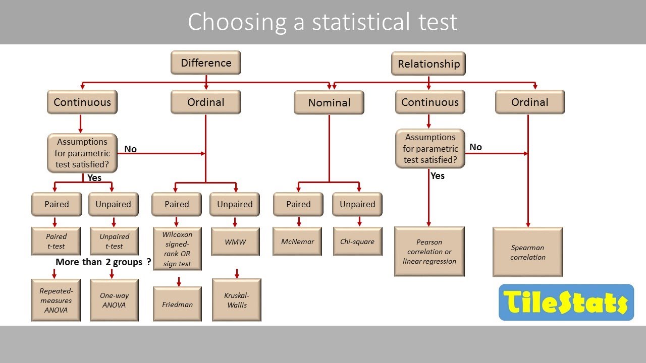
[Music] hello everyone and welcome back today we're going to be continuing our adventure in intermediate statistics and discuss a series of tests um that can be viewed as non-parametrics alternative to tests that you probably already know such as the T test and a Nova test and a couple others as well all right um a couple of them named Cru goal's Conover um we'll also be talking about the Conover Iman test and also the man Whitney test as well so let us get right into it so what do all these tests have in common so all of these nonparametric tests are going to be dancing around the concepts of ranks so what exactly is a rank well we'll give you a few examples of how to find ranks of samples in just a moment but the non alternative hypothesis that we're going to be working with for the kusal Wallace test and also the man Whitney is that the ranks of one population equals the ranks of another population so what do we exactly mean when we say that the ranks of a population are equal so let's assume that the population only has three points just to make it a little bit more easier to see and let's assume that we have a point here a point here and a point here here so let's assume that this is population one and let's assume that we have another uh population let's call it P2 which has points here here and here now notice that I have stacked them directly on top of each other so when they match in terms of value with respect to all the values in this total population of six then we said that the ranks of all of them are equal to one another right so for example we have six points so we're going to have have ranks 1 2 3 4 5 and six generally speaking right but notice that these two have the same exact ranks so do we assign rank one to the top or one to the bottom actually we're not going to assign one or two to either what we're actually going to do is we're going to average those two together to get a rank of 1. 5 and then for the next two points we're going to have obviously three and fours and they're going to be ranked to 3. 5 and then we're going to be looking at those particular values and that's going to go to five and six which are going to tie into 5.

5 so notice that each of these populations of size three will have the ranks 1. 5 3. 5 and 5.

5 for each of their three elements and hence they are equal now some people will say that these tests are synonymous to saying that the population distributions are equal to one another and that's not necessarily true but what is true is if these ranks are equal to one another let's assume that this isn't exactly a symmetric distribution but roughly it is slightly skewed so what you could see here is like xar one and xar two would both be located at the same exact position again even if it's not M part of the set but if you have another distribution of points let's assume you have uh let's assume we have this point here this point here and this point here and again equivalent rank let's assume here here and here notice again even in this example the averages xar one and xar 2 would likely be somewhere located there but notice that the variances of these sets are completely different even though the ranks are equal in both of these examples right so equality of ranks does not necessarily imply equality of distribution because the variances could be completely different even though the ranks match but if the ranks do match then what we have here is evidence that the averages are also equal as well so if we for example look at the average rank of both of the sets um or the distribution of the ranks for example then we would have nonparametric evidence because we're not assuming it's normally distributed um that the means would be equal so this perspective obviously motivates um the idea of a non-parametric alternative to T or zpac test that assumed normality of distributions so let us just formally State out a couple of the goals that we plan to aim in this discussion so our goal is to find non parametric Alternatives alternatives to the following test and most of these you definitely should already know so the first is going to be a t or Z test for two different means and we're actually going to be talking about two non-parametric versions of this the first is going to be called The Man Whitney test and there's another uh known as the Conover Iman test right so those will be non-parametric alternatives for the T test for two means and then we also have the Anova Anova test for three or more means right and the test that we're going to be using for that in the non-parametric world will be the cuscal Wallace and then so that covers pretty much all of the values of means and then we have for example the F test for two variances right so we're going to be looking at how we can actually use ranks for testing equality of variances um which obviously equality of ranks doesn't imply uh quality of variances but we have a couple alternative ways to sort of solve that problem too and we also have for example the generalization of the F test which is of course the bartl test if you've heard of the um other Alternatives um compared to the Bartley test where you know you have slight variations from normality um then actually these test will be a little bit more useful and this is going to be 4 3 plus variances of course and the test that we're actually going to use for both of these um is known as the Conover uh some people will also call these squared ranks test right so we have four different tests that we plan to cover today the man Whitney the con Imon Chrisco Wallis and coner test right so let us just jump right into a numerical computational example and sort of see how we're going to work out these calculations and interpret them so let's start with the basic case where we have two sets I've made the sets relatively small and the numberers relatively nice because otherwise you probably using r or some other statis statistical software in order to analyze this and in R it's not actually not that difficult to implement as well but we can talk about that at another time so let's assume that we have these two sets S1 and S2 that have the elements 5 7 8 9 10 and 12 6 9 13 14 15 15 and 17 respectively so what we want to do or aim to do is do a non-parametric alternative for the equality of two means test which is obviously going to go into either a man Whitney or a Conover Iman depending on your preference both relatively give the same results but you should be analyzing both results and sort of analyze the distribution respectively um on your own um but regardless of which test you're going to do they're all going to start off relatively the same exact way so what we're going to do is we're going to look at all of the ranks for these sets globally right so some people will call these the global ranks so we're obviously going to have how many values here so for the first simple we have we have 1 2 3 4 5 and six so N1 will be equal to 6 and then we have 1 2 3 4 5 6 and seven values for the second element so once we add up those two total we're going to have a total of n is equal to 13 values right so what we're going to do is we're going to have Global ranks 1 2 3 4 5 6 7 8 9 10 11 12 and 13 and in the end if we have any ties um which we do have a couple in this particular is that we have a couple nines repeated a couple 15s repeated at least um then some of these values might not be used and we might be using decimals or if we have a tie of three then we might be using one of these three times or something like that so let's look at the values uh in each of these sets right so where is the least value in these sets right so obviously if you want to do this by hand sorting them from least to greatest it is definitely a must right and also let's keep track of the set either one or two that these values belong to right so what are we going to do so let's actually make this table a little bit more nicer to look at so it's a little bit more easily readable right so what is the least value here so we have obviously a five right so that's going to be the first value and that belongs to set number one uh the next value in sequence is going to be this number six and that's going to be in set number two and then is going to come this seven here and that's going to be belonging to set number one and then we have eight that's also going to be belonging to set number one and then we have two nines so N9 and n and that belongs to set one and set two or you could do set two and one um now since we have a tie for these two we don't want to assign set one to rank five and set two to rank six that's kind of biased right so what we're going to do is we're going to do the average of these two and that's going to give us a rank of 5. 5 and 5. 5 for each of them and obviously now they have the same exact rank in the global settings right now let's continue so the next value after to nine is obviously going to be 10 and that's going to belong to uh set number one and then we're going to have 12 and that's Al also going to be belonging to set number one and the rest of these values are going to be belonging to uh set number two so that's an obvious thing so obviously going to have 13 14 15 15 and 17 and of course we have another tie down here between ranks 11 and 12 even though they belong to the same set you still need to break those ties so we're obviously going to have 11.

5 and 11. 5 for those two values right and obviously 11 + 12 and 11. 5 * 2 still add up to the same total rank um so we're not going to have any issues in that regard so so once you have this Global rank table now what you need to do is place these values of set number one for example into a set of their own and then we're going to have another set for the rank two rank uh the set two ranks right so what are we going to have so the set of ranks for sample one are going to be what so we're going to have rank one rank three rank four rank 5.

5 and then rank seven and then rank eight so all I'm doing here is I'm just grabbing those values for the ranks right so 1 3 4 5. 5 7 and 8 so those are the ranks for set number one and then we're also going to do it for set number two and that's going to be obviously everything that's not circled here so 2 5. 5 9 10 11.

5 11. 5 and finally 13 right so these two sets are going to be very very important for uh setting up a lot of these statistical metrics that we're going to be working with for testing that previously mentioned hypothesis so now let's talk through a couple of the metrics that we need for a man Whitney test okay so let's assume that the size of S1 is N1 let's assume that the size of S2 is equal to N2 and technically speaking you could have several uh different samples let's assume we have G groups here and let's assume that's equal to NG and let's also denote that the sum from I is equal to 1 2G of each of those let's define the total sample size across all groups to be equal to M and obviously that's going to be the uh cardinality of S1 Union S2 Union all the way down to the union with SG okay so the next metric that we need to calculate is referred to as the total ranks the total ranks so the total rank is going to be defined as follows and I'm going to use capital T to denote it and that's going to be equal to the sum from I is equal to 1 to NJ of the ranks of those particular groups so the ranks in set J um each of them right so we're going to take all the values in R1 and we're going to add them together we're going to take all the values in R2 and add them together together so if you sort of continue with the previous example that we have uh with our data sets what you're actually going to find for T1 and T2 you're going to have a total of 80 28. 5 and 62.

5 and you're thinking oh well we have T2 being significantly larger than T1 so does that imply that S2 the sample 2 um is significantly greater than the majority of the values in T1 and you might be right when you say that but keep in mind um sample 2 has more values than sample one so is it possible that T2 is larger only because of the larger sample we don't know right so let's sort of think about how we're going to uh work out those complicated details right so let's assume that we have um a rank of one and then followed by a rank of two in the next sample and then three and then four and then five and then six and then seven and then eight so pretty much what you have here um is like when you interlock your fingers one after the other right so all of the ranks are obviously not equal to each other um in this particular demonstration but they're roughly the same exact distribution one could say right so obviously we don't expect T1 and T2 to be equal to each other even when we do have a relatively ideal scenario as this where you have two sets that are not equal to each other but they roughly have the same exact ranks to one another so what we have here in this pedagogical example is T1 to be equal to 9 and T2 to be equal to 12 so obviously in this particular example this is something that we might want to classify as statistically similar or statistically close to one another right um but that obviously depends because if I have more values in this particular set for example if I add another value here another value here and another value here T2 is obviously going to dominate because it has more values in it compared to the other sample right so let's just take a note uh take a moment and note that down right so if a set has more values in it its total rank so it's rank total TJ may be larger may be larger due to the larger sample size right and that can be a problem right and so it's larger due to its sample size not necessarily its ranks right so here's a question that I want you to think about you might want to pause the video and think about this is how long large can TJ of those total ranks actually be so if you think about it from some things from pre-calculus let's just recall one very cute identity if I take the numbers 1 2 3 4 and go all the way up to n this is actually equal to n * n + 1 / two it's a nice uh very well-known arithmetic uh Series right right so for example if n is equal to 13 for our particular example which was decomposed into a 6 + 7 split for N1 and N2 then what you're actually going to have I if I total up all the ranks for the total set of 13 what you're going to have is that T1 + T2 for sample 1 and Sample two is actually going to be equal to the total of the original ranks if we were to just unionize them into the same same exact sample so that would just be equal to 13 * 14 / 2 which is equal to 91 so for a 67 split for two sample analysis for for equality of ranks the upper Bound for both T1 and T2 is equal to 91 and I leave it to for you to verify that if we take 28. 5 and 62. 5 and add them together you should get 91 right so obviously ly we have this kind of issue right because we don't want them to be relatively small and we don't want these T's to be relatively large even if they had do have larger sample sizes so is 62.

5 significantly close to 91 and is 28. 5 significantly close to zero so we have two equivalent perspectives of the same exact problem so how are we going to deal with the issue where our sample sizes might overtake the value of T right so if the ranks are about equal about equal the rank total should be about equal as well so with this idea some people will create these new test statistics which I'm going to be calling U1 and U2 to be equal to the values T1 and T2 but trying to offset the sample size difference between the two right so if it's really if N2 is really really large when we subtract this total N2 value off it pretty much brings that value of T2 down and we're just going to call that N2 right so we have these U test statistics sometimes referred to as partial partial U test statistics right and for for our example if you're still following these calculations you're going to find that U1 is equal to 7. 5 and U2 is equal to 34.

5 and we still see that the second sample has a test statistic that is significantly large right so now we need to figure out how large is large and how small is small when it comes to these values of U1 and U2 so now let's talk a little bit of statistical Theory and you might want to try and prove these things on your own depending on what you're trying to get out of this conversation but there is one very important theorem and you can take this as axiomatic if you will and it's that these values UJ U1 and U2 will always be between zero so even though we're subtracting something off um it will never result in a negative number and the upper bound will actually be the product of the sample size so that would be the largest value that U1 and U2 can be and there's another very fun exercise if you want to try and prove some of these results and that is if you take U1 and U2 and add them together you're actually also going to get N1 * N2 and that's actually quite interesting and obviously these might be just cute little mathematical facts but it gives us us some idea of how to quantify how large is large and how small is small now we don't necessarily know at least blindly what the distribution of these u values are so let's just call this the UJ axis and this for example the probability Mass function of U and we don't necessarily know what its value is so we can just draw some arbitrary shape there but obviously we don't want U1 or U2 to be close to zero and we don't want U1 and to be close to the maximum value that they can be in particular the product of the two so obviously our rejection region for equality of ranks will be on the opposite tails of this distribution where the lower bound of this distribution is zero and the upper bound of this is going to be N1 * N2 right so for our particular example we actually have these C offs we have 7. 5 as the lower bound and we have 34 . 5 in this particular value right now keep in mind that these are test statistics there for this shaded area in blue do you know what the Shaded area of blue is called this is commonly called our P value Associated to our statistical test now obviously one can say okay well I have our test statistics how do I construct critical values to compare them to um and also how do I calculate the P value because I don't necessarily know what this distribution is in order to integrate it or do maybe a cumulative probability Mass some on that right so let's sort of go ahead and answer that question for us so what to compare these values to in particular these test statistics right because these are partial U test statistics so in the r programming language and python and a couple other also have um ways to calculate these critical values these are associated to a distribution known as the will coxen distribution right and an r that would be q w i l c x and if we're working with a two-tailed test then obviously it's going to be Alpha over 2 and then it's going to ask for your sample sizes M1 and N2 and they can be inputed in any order and then we can do lower.

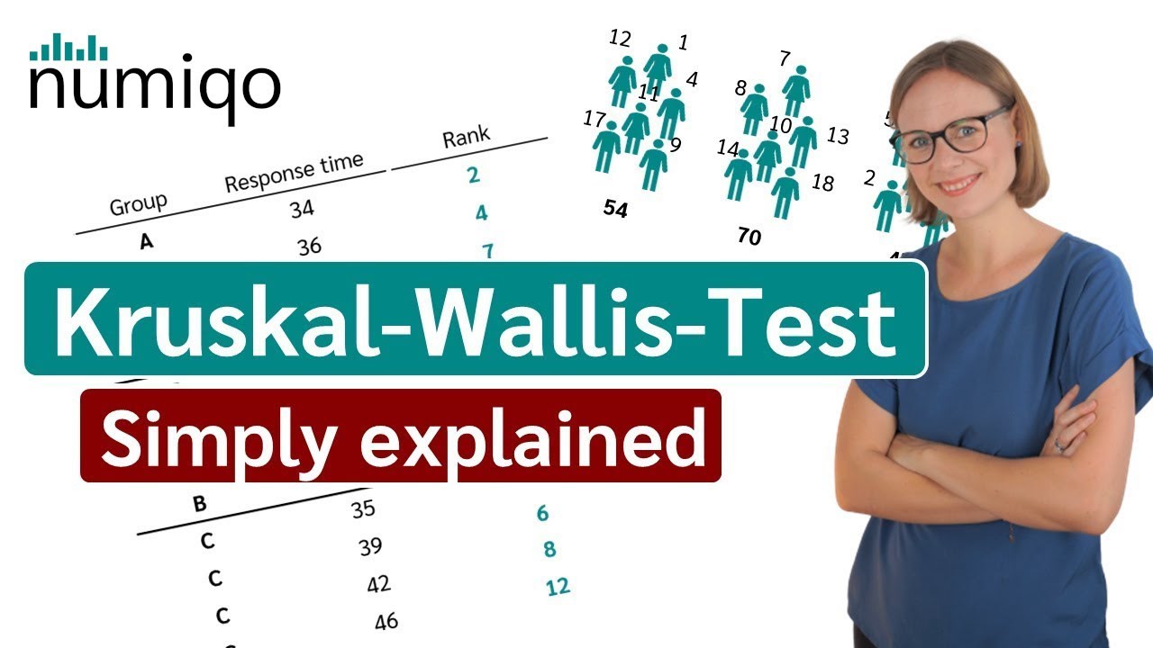
tail is equal to true or we could do lower tail is equal to false depending on the values that you actually want to get right and these are going to give you critical values um Associated to your distribution you can call it say U crit L and U crit W to compare to ustat L and ustat um R for example right so if we choose for example Alpha is equal to 0. 05 which a lot of people do what you're actually going to get is a will coxing critical value on the left to be equal to 7 and a will croxen critical value on the right to be equal to 35 right so where are these values in this table so let's draw this in Orange so 7 is going to be located here and 35 is going to be located above there just to 35 so if we sort of shade this in right so what would this area be so this area is shaded in red that's our Alpha over 2 and that's our Alpha over 2 here and keep in mind how do we get these two values you just switch the true to false or false to True whichever one you did first right and using uh a similar function instead of Q just replace that with p and feed it those Associated test statistics you can also find that the associated P value which according to this picture obviously should be larger um than our Alpha value is actually going to come out to approximately 0. 0514 now if you chose Alpha and then you find the P value obviously your P value is larger so we fail to reject the non hypothesis at least slightly with some weak evidence um but if you calculate the critical values compared to your partial use stats you get the same exact conclusion right and that's looking at things from two angles now there is one very important thing you must note about this so since one moves down for example when I talk about one I'm talking about U1 or U2 the other will always move up and why is that well that's very easy to prove because keep in mind U1 and U2 always add up to the product of N1 and N2 so if U1 gets smaller U2 must get larger in order to still be equal to this product of the samples sizes right so as one moves up the other moves down so technically speaking we should not be looking at a two-tail test here because we already know what the other tail is going to do when we already know what either the left or right tail um looks like in terms of extremity so what is common uh for the man Whitney tests so what the man Whitney test does is it defines as the test statistic instead of looking at both it actually just looks at the minimum of U1 and U2 right and some people will use this instead as just uat to be equal to the minimum of U1 and U2 um and it just looks at the minimum of those partial U stats and then instead of dividing your Alpha over two it just looks at your Alpha value um in the left tail so how small is close to zero um this critical value where it's just one tailed will answer that for you right so that's pretty much how the man Whitney test the two-tailed version and the one tailed version um actually goes right so the man Whitney so the man Whitney obviously since we're only looking at two uh is only used for two groups at a time or you can use it for pairwise pairwise comparisons if you have multiple groups but as you already know pair wise comparisons does come with that downside because every test you do you're going to have a potential possibility of making a type one or type two error um so that's obviously where the Cru scal Wallace is going to enter the story and sort of overcome that particular parir wise comparison issue right so let's actually look at how the crus scal Wallace test is set up just in case you do have multiple groups and you don't want to do pair wise comparison test so now let us consider how we test the equality of ranks across multiple groups in particular when G is greater than or equal to three because if G was equal to two then you should be using a man Whitney test for example right so keep in mind the alternative is that the ranks for um at least two samples are significantly different from each other so even if you have 50 groups um and 48 of them are really similar to each other um if one of the other two are not similar to each other then this is going to lead to a rejection right and then obviously if it leads into a rejection you can do parw comparison test as a post talk test to sort of figure out which ones are significantly different from each other right so how does the crusca Wallace test gr all right so cuscal Wallace so this is pretty much your non-parametric Anova test is going to start off in the following way so we have our sample one our sample two all the way down to sample G now again G greater than equal to 3 we're going to globalize rank all of its values and then we're going to have sets R1 r R2 all the way down to a set of ranks RG and for each of those sets of ranks We're also going to have average ranks for those t uh sets right so we're going to have a bunch of rank sets and we're going to have average rank sets as well right also keep in mind if we have S uh that is defined to be S1 Union S2 Union all the way down to Union SG where the cardinality of s is equal to n and we look at all of the ranks in that particular sample I leave this as an exercise because this is actually really pretty fun to prove this is always actually equal to n + one uh divided by two right so this is a very uh useful thing to keep in mind that the average rank across all values even if you use ties is always equal to n+ one and this is a very very important thing to keep in mind because it actually allows you to shortcut um a lot of these calculations and instead of using r bar I'm going to use R Bar Bar because it's technically the grand mean of ranks which is what I'm going to call it right so how does the crusa Wallace test statistic look like so the crusa Wallace stat some people will use H instead but I'm just going to use uh uh KW for Cru WS because um H is commonly used for something else um the Cal wall stat is going to be defined as follows so it's going to be n minus1 time a fraction of sums right so on the top we're going to have the sum from J is equal to 1 to G of NJ Times the average rank of group J minus the grand rank squared now if you're familiar with the Anova test for parametric testing that assumes normality this is similar to the SSM in the an Nova test the only difference is you replace r barj with X barj and R Bar Bar with xar bar and you get the SSM for your NOA test and on the bottom what we're going to have here is the sum from J is equal to 1 to G of the sum from I is equal to 1 to NJ of r i j the baby ranks of each of the groups minus the grand average squared now some people will look at this as the average of group J but the Cru SC walls and its original form uses the grand rate to compare but nonetheless this object here is also similar to the ssse if R Bar Bar was changed to R Bar RJ right but nonetheless there are similarities between both the original form and that slight variation if we were to change that slight character right now one very beautiful thing about this is we don't actually have to use the will Cox and distribution to get critical values because as each of these ends if each of them are significantly large then what you're actually going to see and some people will use five and 10 as um cut offs but technically speaking it really depends on the scenario uh this dist this test statistic is actually going to fall a Kai squ distribution with G minus1 degrees of freedom right so that's a distribution that we know very well and one can find at least for our example in case you're trying to calculate this our KW set for our two groups even though technically you're not supposed to be using KW for two groups um is going to be approximately equal to 3.

74 if you want to just try and work that out on your own right so is 3. 4 3. 74 large or smaller well it depends um obviously we need to look at a Kai Square distribution um so generally speaking as long as G is uh not equal to two um which it is in this case um is going to look more like this and obviously this is going to be a right tailed test so your Alpha is always going to be in the right tailed area and this value here Kai Square crit is going to be what you're going to be comparing this KW that to in this particular case and keep in mind this is a k^2 g minus1 distribution and I believe when G is equal to two um when the degrees of freedom is equal to one you have a weird case where it sort of like looks like an exponential decay curve um which is why this shape is slightly misleading when G is equal to 2 um because technically you're not supposed to be using it for G is equal to 2 anyway but for our particular example if we do use G is equal to two and that's perfectly okay on the calculation m with one degree of Freedom you're going to have 3.

84 as your critical value right so we have 3. 84 there we have 3. 74 over here um so we're not in the rejection region so we would fail to reject the N hypothesis um that the ranks across all these g equals to two groups are equal to each other right so that's actually very very cool now I just want to mention here once you do have evidence to reject the N hypothesis under a crusco LS then you can use for example pair wise comparison test with the man Whitney test but an alternative to man Whitney for pairwise comparison or two test is known as a Conover Iman test right and the test statistic for con over Iman is actually quite easy so the con over IM or the CI stat is actually going to be defined to be T1 minus T2 so those are the our total ranks divided the < TK of n our total sample size * n + 1 /2 uh times 1/ N1 + 1/ N2 some people will put absolute values here but theoretically you're not supposed to and the reason I say that is because this test statistic if you leave off the absolute values is going to follow a t distribution with N1 + N2 - 2° of freedom and if you take the absolute value can follow T distribution because T goes to negative infinity and absolute value does not right and you might be looking at this and be like oh this bottom obviously would be the standard error of the difference between two ranks but nonetheless this overall object is reminiscent of a pulled variance T Test right so this object here is sort of uh making us think oh is that the the pulled ranks test and I'll let you sort of think about that on your own and sort of see why that is but if you know the formula for the standard error for the pulled variant C test this thing in parenthesis definitely should look familiar and also the degrees of freedom on that right so the con of imen test is actually a little bit more quicker um compared to a man whitne test because one you don't have to do a w Cox and critical value and all you need is the total ranks and the total and the sub uh sample sizes to conduct this right and that's obviously convenient right so that gives us our man Whitney our crus Wallace and this newly introduced con Iman test and all of them assess the equality of ranks for means in the non-parametric banner now let's look at the non-parametric variation of the bleay test so now we look at the non-parametric alternative to the bartl test and the non-parametric alternative is called the Conover squared ranks test so how does the Conover test and how should what is it and how should it be conducted right so what we're trying to look at at now we're still going to be looking at the ranks but we're going to be looking at the spread of the ranks instead and keep in mind just because the ranks are equal does not mean that the spread of those ranks are equal as well right so let us just recall the formula for sample variance or even population variance sort of get an idea of a metric that we might want to construct so the formula for the sample variance for a group J is going to be equal to the sum from I is equal to 1 to NJ of the individual values x i j belonging to group J minus the mean of that group squared all divid NJ minus one so pretty much what it does is it takes each of the values and it shifts them uh about the mean right and then it squares that so what we're actually going to do is we're going to do a a very similar thing now right so keep in mind we have several groups now we have S1 we have S2 and potentially we have more in particular SG of them and keep in mind the coner test can be used for two or even more uh obviously the larger the sample size the better for this so for each of these samples what we're actually going to do is calculate some new metrics so A1 A2 all the way down to Ag and these are going to be calculated as follows so we're going to do the absolute value of the original set S1 minus the mean of X1 the original S2 values minus X2 and that's going to continue all the way down to the set G minus the average of set G so it's pretty much doing the same exact thing as we did for the normal variances so what we have here these eight these are just shifted absolute values so these are just shifted absolute values nothing about ranks has been done yet but once you have all of these values A1 and A2 and A3 then what we're going to do is we're going to rank them globally rank them globally just like we did R1 and R2 in terms of their construction so once we rank them globally what we're going to have is we're going to have sr1 sr2 all the way down to s r g right so these are our shifted absolute value ranks right so that's actually pretty interesting right so these are just the ranks ranks that's a horrible way of writing ranks but it's the ranks of the AJ values globally okay so once we have our shifted absolute value ranks what we're going to do is we're going to calculate a couple metrics so the first value I'm going to call the SS srj now that's a long abbreviation but what exactly is that so I'm going to write down the formula here so this is going to be the sum from I is equal to 1 to NJ so each group is going to have one of these and it's going to be equal to srj each of them squared right so do you want to take a guess of what this sssr stands for so this is the sum of squared shifted ranks so it's the sum of squared shifted ranks um so you can practice calculating this so we're going to have an S ssr1 and an sssr R2 um for our particular samples that we had in the beginning of 23.

5 and 5635 as well so those are fun to implement on your own right so once we have our sum of squared shifted ranks then comes a another metric which I'm going to abbreviate by P SSR or P sssr right so this is going to be just the pull sum of squared shifted ranks value so p is just pulled here and this is just going to be equal to S ssr1 Plus SS sr2 all the way down to sssr G all the way ided M1 + N2 all the way down to NG but keep in mind the denominator for this is just going to be equal to M uh but for our particular example that's going to come out to approximately 62. 85 again that's actually not a hard metric to calculate the next metric that we're going to calculate is called the Conover V metric which is going to then be used to calculate the Conover test statistic and this is slightly complicated at first but let's sort of work with it on our own so this is going to be equal to 1 / nus1 times big bracket here and this going to be the sum from I is equal 1 to n so it's the original values from our original sh shifted ranks so this is going to be SRI I squared right so remember when we took all of our values and we subtracted the average and then we took the absolute value put them all in a set Square them all and add them all that's what this particular sum is equal to and once we're done with that so keep in mind that is an entity we're then going to be subtracting off the total sample size N1 plus N2 all the way down to n and multiply it by our [Music] pssr value and then we're going to square it right and once we do that for our particular example you're going to get 31004 and 68 just to make sure you're calculating everything correctly now we have one more step and then we are done and you might be thinking wow this is really complicated why would anybody come up with this and that's actual beauty of the Conover test and I'll illustrate that and why in just a moment so our final value Co that's our Conover test statistic will be equal to 1 over capital V this this value V here right so the Conor of v and that's going to be multiplied by again big sum so we're going to do the sum from J is equal to 1 to G so we're going to do this for each of our groups so we're going to have SSS R and then we're going to do the J values and then we're going to square each of them divide that squared sssr value by the sample size and that's going to give us some number and we do that for each of our groups and then keep in mind that's one value that you need to calculate and then you're going to subtract that from n times our P sssr value again squared again and once you calculate that that's going to be approximately equal to 1. 15176 so that's actually quite very friendly looking number right so you might be thinking okay um a kind of test statistic of 1.