YOLO11: How to Train for Object Detection on a Custom Dataset | Step-by-step guide

YOLO 11 is out and in this tutorial we'll find unit for object detection on custom data set this guide provide a comprehensive step-by-step work through of the entire process whether you already have your images or you need to find the data no data set no problem we'll start by finding free already annotated data sets for object detection already have images I'll show you how to label them for training and create your Data set next we'll train YOLO 11 model we cover training in two distinct environments your local machine and Google callab once we do it

we'll evaluate the trained model's performance and save it finally we'll deploy the model run it in browser and use it with python SDK we have a lot to cover so let's get started any time that I need to train the model but I don't have the data set the first place I look is roof flow Universe there are already half Million data sets on the website and most of them are for object detection so there is a high chance that somebody already annotated the images that you or I need for training and just scrolling through

the website we can see that those data sets come from different use cases there is some foodball data set there are some medical images some aerial images there is data set to the detect fire and smoke there are some data sets related to video games and Data sets to detect safety equipment and as a matter of fact the data set that I will use today in this tutorial also comes from roof flow universe so some time ago I got interested in document understanding and I was curious if I will find a data set that will

help me out to process arive uh papers and that's how I found this TFT ID data set and the cool thing is that you can go into those images take a look at the annotations evaluate the quality and Yeah that data set is exactly what I needed to make this tutorial like I said many of you probably already have the images or plan to collect them you may scrape the internet or take images with your phone or scan documents and if that's the case let me quickly show you how to annotate them there are of

course multiple options on the market some of them open source like cat or my open source project called Mak sense but if you're Looking for something that is free to use and with minimum hustle roof flow is probably your best option and of course I don't say that because it's roof flow YouTube channel you can totally trust me on that no but honestly I think it's the best so let me show you how to use it so for the next few minutes I will will pretend that I don't have the data set that is fully

annotated already and I will use the sap set of images from TFT ID data set to guide you through the Whole labeling process the first thing that you need to do is to log into your roof flow account or create one if you don't have one already and once you do it you will probably end up in this main workspace view here I click the new project button that is in top right corner and that takes me to project creation view now I can provide the project name I'm just replicating the TFT ID data set

so that's the name that I'm going to use and I need to provide Annotation group this is pretty much the answer to the question what objects am I going to annotate and in my case those are going to be research papers we select project type here object detection and create a public project the first thing that you should do once you create a fresh project is Define the list of classes that you would like to annotate like I said I replicate TFT ID data set so in my case I will use figure table and text

once you're happy with The list of classes you can click add classes button success yay great successful and now the next step is to upload your data to the project to do that we go to upload data View and here we just drag and drop our images and and once we are happy with the list of images that you would like to add to your project we click save and continue depending on the size of those images and the amount of images that you uploaded that process can take between Few seconds and few minutes the

next view allow us to pick the way that we are going to annotate the data set you can use the auto annotation uh functionalities that are in roof flow but for this particular data set I don't really recommend that we can hire somebody to annotate the data for us or we can manually annotate the data set and this is the option that I'm going to use here that view will probably look a little bit different for you uh I have a Lot of people in my workspace and I can just invite them to help me

with annotation but uh for this particular job I will just assign uh those images to myself and here it is our first annotation job is is created and I can just start annotating uh so I click Start annotating button this takes me to the editor where I can move between images and let's say that I would like to Annotate this one I just zoom in I draw the bounding box around the object that uh is interesting to me I pick the class I submit and I just do it for every object visible on the image

so I had uh two more text Fields one more table uh over here here and one more text uh below the table I try to make all the bounding boxes uh consistent so the padding around the object is the same here is another a page from uh a research paper Uh a large uh text field um here's another text and below it uh there is a small table so just zoom into it uh to make sure that we annotate everything nicely there it is table and here is another text let's pick the class great I

hope that you get the idea already and once you annotate all of your images you will end up in this approve reject view where you can for the last time take a look at all of your annotations make Sure that they are right before adding the images and the annotations to the data set I annotate all of those Imes myself so I will just click add all but you can be more granular and add or reject specific images once you do it you can add your approved images to the data set this will take you

to this uh view where you can select how many images would you like to put in your train validation and test subsets I will just keep the default ratio of 7021 and Add those images and the last step is to create a version uh when you create a version you can apply processing steps and augmentations and for this specific data set I will skip the processing steps I will even remove the resize only keep the auto Orient and I will not apply an augmentations as I work with documents so I don't want to flip them

rotate them or I don't know uh Shear them so I skip all of those but for your specific use Case uh those might be useful click continue and create and depending on the amount of images and their size that creation step may take a little bit of time but once it's completed you finally have the data set that you can use for training and to do that you will Cate uh you will click the download data set button pick the export format that you would like to use in our case that will be yolow V1

and download but I will cover that step during the training Process we have the data now it's finally time to train the model I will be using Linux machine with Nvidia GPU and I will perform most of the configuration and training using terminal interface if you don't know Linux commands don't be scared I'll try to explain everything along the way and spell out what's happening if you're using Windows make sure to use WSL uh windows subsystem for Linux it just provides a more consistent And compatible environments for running all the tools and scripts so here

we are in Linux terminal and the first thing that we are going to do is to create a separate directory uh for our tutorial so I navigate to documents using CD command change directory and once I'm inside I create new directory called uh YOLO 11 tutorial and once again I go into that directory inside I create new VM and for those of you who don't know VMS allow you to uh Work on different python projects um in parallel you can have different uh python version in each VM you can have different versions of your dependencies

in each VM and those versions uh don't clash with each other and uh once I'm inside uh I activate uh that VM now every python related command that I am going to run will be executed in context of that specific vmf our python enironment is ready now it's time to fill it with all The necessary dependencies to train YOLO 11 model you will need ultral lithics package and one of its core dependencies is pych if you don't know pych is probably the biggest machine learning framework right now used to research and deploy neural networks like

YOLO 11 for example and to run efficiently it's actually very close to your Hardware that means that you have different installations for CPU and for NVIDIA GPU and for Amdgpu and to make sure that everything is configured properly ultral ltic documentation actually recommends you install pytorch separately on your own and let me show you how to do it the easiest thing you can do is to go to p.org website and scroll down a little bit they have this really cool uh installation command generator where you can choose uh your operating system and the hardware that

you are using and the command changes dynamically depending on Your configuration I'm just picking uh Cuda 11.8 and I will tell you why in just a second I copy the command and we go back to the terminal so as you hopefully noticed the structure of the installation command uh was depending on the Cuda version that I have installed uh so um let me show you how to check the Cuda version you have there are multiple ways to do that I will just uh use Nvidia SMI or Alternatively uh nvcc version and my version of Cuda

is 11.6 this is pretty old uh Cuda version it's actually uh so old that in that uh command generator that was on pytor org uh website there was no command for um Cuda 11.6 but the latest version that was there was 11.8 fairly close so what I did is I copied the version for 11.8 and now we will will do small edits to make make sure that it will work for Me so I paste it in the terminal and I change the end number uh in the URL from8 to6 but probably already guessed it's means

11.8 and 11.6 uh and I will do few more edits so I will remove torch audio because we are not working with audio today and I will remove the free at the end of Peep free install uh because I can just use peep within uh my python uh virtual environment now I click Run and uh yeah depending on your internet connection depending on the on the individ individual GPU that you have execution of that particular command might take a little bit of time so uh let's use the magic of Cinema and and skip the installation

once the installation is completed uh we can use a peep list to list all the dependencies that are installed in our python environment uh and we can see that torch And torch Vision are both installed with support for Cuda 11.6 exactly what we need and now we can uh just install uh ultral litics peep package so we type peep install ultral litics uh press enter and here just before depending on your Hardware depending on your internet connection the installation might take a little bit of time but significantly less than than pytorch probably the largest dependenc

see over here is open CV uh but yeah all around the installation of ultral ltic once you have a torch already shouldn't take like more than 30 seconds we see that it's already wrapping up and yeah once it's done um it's good idea to run uh YOLO help just to confirm that the ultral litic CLI works as expected looks like our python environment is ready now it's time to download the data set as I said before I'll be using this TFT data set that hopefully will allow Me to train model to detect text figures and

tables in research papers and to download it I navigate to a data set section click download data set button pick the export format that I want to use in our case uh yellow 11 and for the local training uh I'll be using uh the zip file so I uh check this uh radio button and click download and depending on the size of your data set that might take a few minutes to complete once the download is completed I'm back into the terminal and the first thing that I will do is confirm that our ZIP file

with our data set is in downloads directory and to do it I will use LS command with two options l and a so I will use a option to print all the files and I will use l option to do it in the long description format and then I will look for files that have TFT string in their name remember our data set is called TFT ID and that's uh the grab command and the pipe in between Those commands is used to stream the output from the First Command into the second command so that I

can chain them and indeed there is a TFT ID zip file in our downloads directory so the next thing that I will do is I will create a data sets directory inside my current directory so inside YOLO 11 tutorials and I will go into that directory and then I will copy our uh TFT ID data set zip into my current Directory I can confirm that the copy operation was successful by just listing files in my current directory uh indeed there is our ZIP file over there now I will use unzip command uh to extract files

uh from that zip directory uh and I will use once again two additional options the first one is Dash Q to make it quiet because by default unzip list all the files that are extracted and we have thousands of files and another one is dasd to specify The target directory uh and now uh I will try to take a look inside the target directory to uh understand the structure of uh my data set and to do it I will use the tree command um tree command also has plenty of options but first I will use

dashd stands for directory so uh This Way tree will only display directories inside directories um and on once we execute that command we can see that we have Three subdirectories train test and valid those of course stand for the data set splits and each of subd directories have two more directories in them so we have images and labels inside each subdirectory and uh this is the this is the structure of the data that you need to maintain for ultral litics to understand how to load your data set during the training and to be honest it's

very similar to the structure of Data that we know from the previous versions of Yola model now the next step is to go beyond directories and to understand the file structure so another option uh that we can use in uh tree command is uh Dash capital L that stands for layer of the tree so we can decide how deep we want to go and and this time I'm am using uh-h L3 so that I won't go inside images and labels Subdirectories because like I said before we have thousands of of files in those subd directories

so those would just flat our uh terminal and we wouldn't be able to see anything so uh we see free files inside TFT ID data set there are two RMS that I don't really care about and there is one data yam file and that file is certainly interesting to us and I want to show it to you but before I'll do it let me just switch that uh dl3 into- L4 to show you The amount of data that we have in those directories so we see that we have uh over 17K files uh inside data

set which is interesting yeah because we only had less than four less than 9,000 images but somehow we have uh 177,000 um files inside the data set and I will I will explain why is that in in just a second but first let's take a look at the at the data yaml file uh that I told you about uh a second ago so To take a look inside files we can use cat command cat pretty much prints the content of the file into the terminal so I'm I'm using Cad and specifying the path of the

data yam uh file and uh we can see that's pretty uh typical uh yaml file inside um not very long um so let's take a look what do we have here so first of all we have a train Val and test keys in that uh yaml file and those um specify relative paths to the train test and valid subd directories or Actually to directories storing images inside those sub directories to be precise um that I showed you just a second ago next we have NC that stands for number of classes I believe and in our

data set we have only fre classes and the next one is uh names and this is pretty much the list of the classes uh that we have in the data sets kind of redundant information you don't need the N see if you have the names but whatever um okay so now let's take a look at Those files why do we have 17K files uh if we only have less than 9,000 images so let me first least all all the images inside the train sub directory or uh even better let's just uh print the first 20

images for that we can use the head command and we can just specify the number of U entries that we would like to show um and because uh things are ordered alphabetically when you use LS um this order is constant so we can just Print the first 20 line and this is always be the same 20 lines um and once again I'm using the pipe to stream the output of the First Command into the second command um you know what let's uh drop the LA uh to make uh the representation a bit more concise concise

I'm only interested in the in the names awesome and now we can open new terminal window I will just move move it uh over here and here we will display the Content of the labels directory from the train split uh so just before I will only show you the first 20 files uh from that directory and uh if we will take a deeper look we'll notice that the names of the files in the images directory and the labels directory are the same the only difference is the file extension so in the images we have jpex

and labels we have txt files and you can see that the first file have the same name if we will take a deeper look the second and the Third um have the same name as well and the last file also have also have the same name so now let's copy one of those names let's go back to our original terminal and use cut once again this time not to display the data but to display the content of that labels files and once we do it we see a bunch of numbers what do they mean let

me show you okay so I went ahead and I copied the first three lines from our annotation file if you would take a look At the original file it had like 10 lines in it but three lines is just enough for me to explain how yellow annotation format works and I also rounded all floating Point numbers to second digit after the comma for those of you who are unfamiliar with u software engineering jargon floating Point numbers are just the numbers where we have some digits after the comma and two digits is once again just enough

for me to explain how the whole annotation Format works so in yellow annotation every line describe a single bounding box along with a class associated with the bounding box so we have four floating points numbers that describe the position and the size of the bounding box and we have one integer that describe the class ID of that particular bounding box now those numbers in the txt file are separated by a single space and they form kind of like this Table so the First Column from the left is actually the class ID now what is class

ID that's a convention that we use in computer vision so for example in our data set we have three classes figure table and text those are the class names but in practice turns out it's often a lot more convenient to use number representation not that text representation that's why we map those class names into class IDs those are integers starting with zero up to n Minus one when n is the amount of classes that we have in our data set so in our case Zero maps to figure one maps to table two maps to text

so anytime that we will see a line in our annotation txt file that starts with digit two that means that the whole line describe a bounding box associated with text class now we have four more columns uh starting from left to right those are X Center y center with and height of the Bounding box so it's a little bit weird that we use X Center and Y Center to define the position of the bounding box but this convention is uh is coming back probably to the first YOLO uh model ever uh and it just uh

stayed the same uh through the the years now important thing is that those numbers are normalized so X Center y center with and height of those bounding boxes that were initially expressed in pixels got divided by respective dimensions of the Image uh so that in the end uh the values are between zero and one now that we have our python environment ready and we understand the structure of our data said it's time to start the training you can do it in two ways using python SDK or the CLI but for the purpose of this tutorial

I'll be using the CLI option but before I trigger the actual training let's run YOLO help command to understand the structure of the command we need to Start the training so we see that every command and ultral litic CLI have this YOLO task mode and then additional argument structure and if we go to ultral litics documentation we can see that values for the task may be uh detect segment classify pose and obb this stands for oriented bounding boxes in our case we are going to use detection and the mode can be train validate predict export

track and Benchmark in our case this is Going to be train if we scroll a little bit lower we can see an example of uh detection training command with some of those additional arguments specify the most important of those are data this is the path leading to data yam file the file that we saw just a few minutes ago and model this is the name of the checkpoint that we are going to use to start the training there are also some additional hyperparameters that I will discuss in just a second But before we do that

let's talk a little bit more about the checkpoint options that we have so every task have five checkpoints that you can use ranging from Nano to X and those checkpoints uh differ in sizes so the amount of parameters the model have but also the expected map value in that table we can see values on Co data set so YOLO 11n have significantly lower expected map value than Yol 11x and that's Something that you should keep in mind when you will uh choose the checkpoint for your training I'm using YOLO 11n but I'm only using that

because I want to have small model so that it trains fast during the recording of the tutorial in your case you might actually aim aim for something bigger than the Nano version so now we are back in terminal and we can finally start the training so what I do is I type in Yolo detect train Command and I provide additional arguments like we saw the first one should be data and here I provide the path leading to data yam that is inside the root directory of my data set the next one is model and here

like I said I will use YOLO 11 Nano version I also specify two more hyper parameters EPO and set it to five an image size and set it to 640 I will tell you more about those hyper parameters in just a second I Trigger the training and it fails and when we examine the error we can see that ultral litic c complains about in correct path leading to validation images and this is the error that a lot of people experience so let me show you how to solve it the first thing I do is I

navigate to the root directory of my data set so go to data sets TFT ID and then I run PWD command this is the Linux command that shows you the global path of the directory that you're in and I Just copy the result of that command and we will edit the data I will do it using Nano this is the command line editor but you can use vs code pretty much any text editor that you have and what I do is I update the paths to train test and validation subset and I remove those two

dots and I paste the result of PWD command essentially what I do is I change the relative paths to Global Puffs once I finish I close I save the file I can confirm that the file was Updated by just using cut data yam command that we already know we can see that paths to train test and valid subsets are now global and now what we can do is we can go back and restart the training so I just run the same command hit enter and the training starts uh we see a lot of high hyper

parameters um that either we defined or are set to default values you can see uh the summary of the uh model architecture and we see that the training runs now What can we do to monitor our training so let me go back to the second terminal window that we had open and the most OB obvious thing is to run Nvidia SMI here we see the GPU usage but this is only the snapshot of of the uh GPU usage that was registered at this specific moment in time and if you would like that uh Nvidia semi

command to be updated constantly what we can do is we can you use watch uh this is the command that reruns the command all the time and we Set the update period to 10th of a second this way we have this kind of like real time um training monitoring showing us the uh usage of our GPU by the way this Nvidia SMI plus watch combo gives you very basic information about your training job so if you would like to know more there are other tools that you can use two names that come to my mind

are Envy top and GPU stat so you can visit their GitHub Pages learn how to install them and this way you will Know a lot more about your training job but also about the behavior of your model and the GPU memory allocation during the deployment the model is training so let me use this time to tell you a little bit more about those additional arguments that you can pass to training command we only set four of them model data EPO and image size you already know what model and data is so let me tell you

a little bit more about the rest of Them starting with EPO a single Epoch of training is model going through every image in your training set so when we set our EPO to five that means that our model will see every image from our training set five times the more EPO you set the longer the training but potentially the higher accuracy of the model you train image resolution is the resolution of the image used during the training but also during the deployment of the model so before the image go Through the model it gets resized

to some predefined resolution uh this is because in your training set there is a high chance that your uh images have different resolution so you resize all of them to a common resolution that you will use during the training now if you set the image size to a higher value you will have a higher chance to detect small objects but the higher the image resolution the higher the memory allocation your model will Need to train uh another argument uh that have similar outcome is the batch size so when I said that the epoch is a

model going through every image in your training set the model does not look at every image separately it looks at multiple images all at once and the batch size regulate uh the amount of memor the images that model will see at once so when we have thousand images in our training set and our Epoch is set to 10 for example the model will need 100 Iterations to go through each image in the training set but when the batch size is set for example to 50 it will only need 20 iterations to get through all of

those images in the end increasing the speed of the training but also like I in said increasing the memory allocation another interesting uh parameter that we see on that list is device uh we can for example use this parameter to use multiple uh gpus for training of a single model I only have single GPU so I Didn't use it but if you have multiple gpus you can speed up the training uh this way uh and people who have Macs for example can uh use a device argument to specify that they would like to use MPS

so the Apple silicon uh rather than the regular CPU for the training or deployment and probably the last one on that list that I think it's uh really interesting is the patience so patience the parameter that you can use to uh stop the training um So the model is actually constantly evaluated during the training and we can use the patients to stop the training if we see no progress during the training so if for for example for 10 Epoch the accuracy of the model did not improve there is a high chance that it won't improve

in the next 50 Epoch so we might just as well decide to stop the training right now and save some time and uh save the money that we would use for the training uh as you can see there are a Lot of other parameters that you can uh choose during the during the training so I highly encourage you to go through that list look for something sounds interesting uh try different values um and experiment okay we are back in terminal and we can see that our training is almost done uh we are just performing the

final evaluation of the model and it's completed and we can see that results of the training have been saved To runs detect train to directory so let's run ls- la on our current directory and we see two things happened first of all uh YOLO 11 n. PT file was saved this is the checkpoint that we used to initiate the training and it was just cached locally so that if we would rerun our training job we wouldn't need to download it once again but also there is a new directory created called runs and this is the

directory that is created by ultral Litics CLI during the training and if we will run 3-D on this directory we'll see that inside we have detect subdirectory and inside the detect directory see another train and train two directories so why do we have two train directories it's because our first training job actually failed remember we did run YOLO uh detect train command but it failed because it couldn't locate all images from validation set but because it did Run uh the train directory was created and then when we rerun uh the command to train the model

once again another train tool directory was created so if we would I don't know um update the hyperparameter and run the train job once again another train free d Dory would be created and we have this detect directory because we did run detection task if we would run another training job but for segmentation we would have detect and segment subd directories in The runs directory now let me open runs detect train to directory so we can examine the artifacts that were saved there during and after the training so the first thing that we see is

the weights directory the first one from the left and inside uh there are last PT and best PT files those are the weights that were saved uh during an after the training but uh we'll play with them in just a second for now let's focus on uh other Assets that are in this directory and the first thing that I want to take a look is the confusion metrix so this is the chart that helps us to understand how many false positives and false negatives happened during the model evaluation after the training but also whether the

model confuses classes so whether the model detects the object but fails to assign the correct class to it and from this chart we see that the model has pretty much only one weakness And this is uh false predictions of text class that means that the object detect text where there shouldn't be any text and that's uh probably related to short training time so if we would have maybe 10 Epoch instead of five we would be able to optimize uh the model in this specific Edge case another interesting artifact is results.png so uh like I told

you during the training the model is constantly being Evaluated and uh we use multiple different metrics to do that and uh on this chart we see values of all of those metrics after every Epoch and we can see that at Epoch number five uh box loss for rain was still higher than box loss for validation that means that our model is most likely undertrained and we could easily train it for 10 20 EPO longer and it would still be uh not overfitting uh and the last uh thing That I would like to take a look

is uh Val batch results so uh those are uh bounding boxes representing detections that happen during the evaluation of the model at the end of the training on the validation set and here I mostly look for things that are clearly wrong something that uh I can visibly see and maybe do some adjustments in my training set to improve on those specific edge cases but here on this chart I don't see Anything clearly out of ordinary we finished the training we evaluated the model now it's time to put it through the test since we trained a

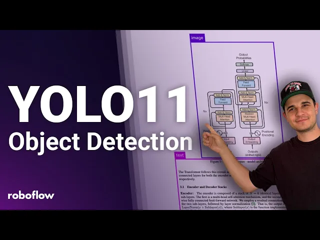
model capable of analyzing research articles let's use it to process some ml papers it would be awesome to use it to process a paper talking about YOLO 11 but traditionally ultral lithics did not released a paper along with the model so I got creative and picked another iconic paper for us to use let's check how our Model handles detecting text tables and images in attention is all you need paper okay so I did found attention is all you need paper on the internet uh it's in PDF format so let's download it uh to our downloads

directory and once we do it let's go back to the terminal and first thing first let's confirm that it is uh really in the downloads directory so let's do ls- la on downloads and this time grab for PDF Files and yep there is only one PDF over there that must be our attention is all you need paper so now let's copy uh the paper from downloads into the data sets directory that we created at the beginning of the tutorial and inside the data sets let's create test directory what I will do now is I will

convert that PDF into range of PNG images and I will save them into this test directory and to do it I will use a little bit of image magic so image magic is a uh Command line tool is a package that helps you to do crazy things with images and it's not really related to the topic of this tutorial but the command that you see right now on the screen will help us to convert that PDF file into uh a list of PNG images and we'll save that to our test directory we'll do a lot

of things along the way like removing the alpha Channel and setting the background color uh to White and uh once that will Happen uh we will uh run the inference on those images if you are interested in image magic I highly encourage you to visit their GitHub page um the docks are crazy uh so it's not easy uh to learn that tool but it's very powerful now let's uh take a look at the images that we generated so let's open that directory in the UI and we see that we have separate PNG file for every

page and can see this iconic U Transformers diagram um on the page three okay so now We can go back to terminal and run uh detection uh through the CLI so once again we do YOLO detect but this time we set the mode to predict we specify few arguments the first one is source and here we pass the path to our tests test directory this way we uh say that we want to run the inference on every asset that is in that directory so on every image and we also specify the model that we would

like to Use in our case we will use the best model we got from our training job so we do runs detect train to weights best PT and then when we run it we see that the CLI shows us uh what classes and how many instances of every class uh were detected on every image and we also get an information that the results were save in runs detect predict directory now we can just copy that path and open it in the UI to take a look we can open the first image from The left this

is the title page it it's a little bit unfortunate that ultral litics uh decided to use why white or almost white color to represent this class but we can still see that sections of the text were correctly detected take a look on another page and yeah we we managed to to detect this iconic Transformers diagram on page three looks like it works now let's switch the environment and let me show you how to run the Training and evaluate the model in Google collab as usual The Notebook for this tutorial can be found in roof flow

notebooks repository where we store demo notebooks for all our YouTube tutorials the link to the Google collab for this notebook will be also included in the description below the video here we just need to scroll a little bit lower to uh model tutorials table and look for YOLO 11 object detection Then click open and collab button once we do it we'll get redirected to Google collab and before we start the training we need to take care of few setup steps the first one is to add roof flow API key to the secret step so uh

to get roof flow API key you need to sign in into your roof flow profile or of course create one if you don't have it yet and then go to settings API keys and here we copy the private API key once we are back to Google colab we open the secret stab that is in the left side panel of Google collab and we add new secret call it roof flow APA key uh without spaces with underscores um and all capital letters and enable the access to that um specific secret um so that we will be

able to use it later on now of course I have my API key set already so I'm just closing uh this tab and the next step is to confirm that we have access uh to the GPU and similarly to the Lo training to do it I run Nvidia SMI uh and here what we can see is U the version of the Cuda that is accessible in uh this environment if you don't see similar output maybe with different Cuda version or different GPU uh what you need to do is you need to open runtime then click

change runtime type and most likely uh you you are on the CPU version of uh Google collab so you need to choose one Of the accessible uh gpus I'm using Nvidia L4 but I'm pretty sure it's not accessible on the free tier so if you are on the free tier just uh choose uh T4 GPU click save and restart the notebook if you set your secrets uh they should uh be still there so it's only to get the access to the uh to the GPU the next step is to install uh the required dependencies so

on a local before we installed ultral litics we need to install py and we needed to make sure That the py version is right for our Cuda over here in collab uh the pie torch is already installed so we don't need to install it what we can do is run PE least and grab uh to look for pytorch and we see that that both torch and torch Vision are installed and in both cases they're installed with the Cuda support so that's perfect all we need to do is run uh install ultral litics and install roboplow

uh because here we will use ultral litics uh to run the training But we will use roof flow to pull the data set from Robo roof flow universe so far we only downloaded the data set as a zip file let me show you how to do it using roof flow SDK so just like before we select data set in the left side panel but this time when we click download data set button and select the uh appropriate export format we will select show download code instead of download zip to computer and once we do it

and click continue the Code snippet will get generated uh I'll just copy the last three lines of that code snippet but if you want the code snippet that will install roof flow SDK give you your API key and download the data set all at once can just copy that paste it in the collab and execute I will just go back to coll up and update those last three lines of that code snippet execute the cell and downloading of the whole data set will take a little bit of time as a Matter of fact according to

uh what we see on the screen will take around 3 minutes so let's use the magic of Cinema to speed up the whole process okay our data set is downloaded so now we can open uh the file browser in the left side panel and take a look at its structure uh we did that already for local training so this time I will go very quickly and only talk about the most important things so the data set have three subdirectories uh test train And valid and a data yam file uh that um provides the most important

metadata about the data set at the very top of the uh yam file we have uh three keys test train and valid those um store uh relative paths to images directories that are located within each subdirectory so now if we open those subdirectories we see that each of them have images and labels uh directories inside and if we open one of those labels Directories and click on one of those txt files we see a typical uh YOLO annotation format we spoke a lot about that format uh in the section covering local training so if you're

interested feel free to use the chapters you will learn a lot more our environment is configured our data set is downloaded so we can start the training but before we do that let's open the resources tab that is on the right right side of Google collab we'll use it to keep track Of the GPU vram usage uh during the training and by the way over here we see that the total amount of vam that we have at our disposal is 22.5 uh gabt so it's actually a fairly large uh GPU and like I said if

you are on a free tier you wouldn't have access to it but I use it uh to uh experiment a little bit so contrary to what I did on a local here I will uh train the same model but uh twice as long when it comes to EPO but probably faster when it comes To time as I will set uh EPO to 10 but batch size to 128 and I can do it because it's a fairly large GPU now I just hit enter and start training just like on local we see the list of all

parameters uh along with values the definition of the neural network and when we scroll lower we see that our train and validation sets are being uh loaded uh and the training should start In just a matter of few seconds and once the training starts we'll see a drastic Spike on the GPU vram uh usage chart so the first Epoch have just started and the spike should happened right now exactly so we see that uh immediately we allocated 17.4 uh gabes of that uh vram and the single Epoch takes around 1 minute to complete and we

uh will run 10 of them so let's use the magic of Cinema once Again uh to speed up the process uh the training have uh completed and we see that the artifacts were saved and runs detect train directory so now let's use Linux LS command to list all the files that we can find there and uh display few charts that will tell us a little bit more about the quality of the model that we trained so the first chart that I'm interested in is the confusion metrix so if you uh saw our local Training um

we had a small problem with the model that we trained locally it had pretty much one weakness and those were false uh positive for text class and back then after five epochs of training we had over five 00 maybe even 600 of those false positive on the validation set and here we see that we've just uh changing the EPO count from 5 to 10 we managed to lower that value below 400 so the model is significantly better at not producing those false detections the Next chart um that I'm interested in is the results PNG uh

one where we have um the values of all the important metrics that were collected during the training here the most important metrics is box loss both for train and validation set and we can see that the Box loss for train is still higher than the Box loss for validation so we can see that the model is still not overfeeding you could still probably uh train it for a little bit longer and It will probably produce even even better results and the final thing that I always like to take a look at is a uh subset

of predictions from the validation uh batch uh just as a sanity check to look for anything that is clearly out of ordinary but uh similarly to the local training I don't see any problems with this model and as a final step we'll run our c in uh validation mode so what will Happen is we'll load uh our freshly trained model into the memory and we'll run it against images from the validation set to compute the map 95 metric for each class and for all classes collectively this is the most popular metric uh to Benchmark object

detection models and we can see that in all cases we crossed 90% this means that at least on images from the validation set the model is uh handling that very well and it's capable of detecting um Images uh text and tables with high accuracy we know that our model works well so now it's time to save it this is especially important if you run your training in Google collab because Google collab environment is only active for several hours and once that time pass all files that were accessible in that environment will be deleted including your

freshly trained model so of course you can download that file to your local that works especially if you have only One project that you plan to work on but if you have multiple projects I guarantee in three months time you will not remember what have you done and in what project so I actually recommend you upload load the weights to roof flow and let me show you how to do it so I'm not sure if you remember but we actually trained the model on the data set I found on roof flow universe so before we'll

be able to upload our weights we need to Fork that data set so That it will be assigned to my account and then I will be able to tie my new model to that data set to do it I go into images and click for data set beta button and once uh that happens the forking process is triggered depending on the size of a data set it may take more or less time but my data set is fairly large um so it will take a little bit of time but once that process incompleted we'll end

up in this view so this is now my data set I can for Example change the name of the classes here I can upload more data I can annotate more data so that gives me a lot of options especially if I would like to improve uh the model that I just trained but importantly it allows me to upload my newly trained model into this project so let's do it at the bottom of uh the Google collab you will find a code snippet that shows you how to upload the weights to roof flow universe but that

code snippet assumes that you Are the owner of the project that you use for training and in our case that is not the case I use the project from roof flow universe and I just created the fork and I would like to tie the model to that fork so to do it I will just paste this code here uh this way we will use rlow SDK to load the metadata of our fork and now we'll just uh make a small updates in the code snippet uh switch the version to our project and uh run the

cell now the weights are being Uploaded into my Fork I can click uh this uh link that is displayed and this will take me to the page where the model will be loaded depending on the size of the model uh you uploaded that might take a few minutes to complete but once it's completed this view change into something like this and now we have a lot more options first of all we have all the metadata of our training but we can deploy the model in all uh different ways let me show you how it works

I will Just uh take one page from attention is all un need paper and we uh drop it here and immediately the model will get loaded into the memory uh of the of the browser because it will run locally I'll run inference on that file and we can see that just as in the case of local the model is capable of detecting both the figure and the text on that page awesome don't get me wrong running your model locally in browser is cool but uploading your rats to rlow allow you to Do so much more

depending on the use case that you're trying to solve whether or not you train the model to detect animals or parts that are manufactured in the factory you can for example deploy that model on small Ed device like this Jetson Nano and run your inference directly in the forest or in the factory to lower the inference cost and the latency you can for example deploy it on phones or in the cloud or you can deploy your model in collab and That's exactly what I will show you right now and we are back in Google collab

I know long time no see uh but this is actually a new Google collab separate environment I created this so you can be sure that the weights are no longer here the weights are actually in roof flow universe and we will pull them to do that we start by installing two python packages that we are going to use the first one is inference that we are going To use to pull the model and run it locally the second one is supervision that we are going to use to visualize the result of our inference one once

once the dependencies are installed we need to make sure that we will have access to roof flow API key this is the same key we used before to pull the data set from roof flow universe or to upload our weights and now we will use it to pull our model back into fresh Google collab environment uh I will copy that Code uh and close the tab paste it here and now we'll use Google collab SDK to extract the value of roboff flow API key from secrets into the constant so to do it we'll call user

data get and pass the name of secret we would like to extract in our case it's roof flow API key all capital with underscores instead of spaces now it's time to pull the actual model to do it we will use a get model function that we need to import from inference Package and uh to pull the model we need the API key but we also need model ID and we will get that model ID from roof flow UI from the page that was created when we uploaded the model okay so we just copy this string

and go back to Google collab paste it as model ID and now we are ready to load the model so I just create new variable call it the model and call get model function pass model ID and roof flow API key hit enter and After a few seconds the model uh should be loaded and now what we can do is we can test the model uh on some example image and I'm just lazy so at this point I will just upload the F page from attention is all you need paper so that it will be

accessible in uh Google collab environment and we'll just use open CV to load that page as uh the number array so let's do it so first thing first I import open CV so we type Import CV2 and now I will Define uh a new constant um image path copy the path to our uploaded image uh past past it here and uh create a new variable called image uh run IM read function from open CV pass our image path hit shift enter and now the image is loaded into the memory the next step is to run

the inference so I create the results a variable uh run model infer function pass the image along with the confidence level let set it to 0.4 and that uh would uh return a list uh by default so I just pick the first value from that list here is the results object um that we got so now we will use uh the supervision to parse that result and display uh the bounding boxes on the image so we import supervision as SV and we SV and now uh we will create a detection object from. uh inference Result

so we create variable called detections uh call sv. detections from inference from inference and now we will pass our results object uh into uh that function and as a result we'll get the detections object so uh the results object and the detections object store the same information it's just detections is the object that we can use to um pass to all sorts of different utilities that we have in Supervision uh next I always like to create a copy of the original image before I annotate anything on that image case I will mess something up and

first thing first I will run a box annotator to draw bounding boxes around the detected uh objects you just pass the annotated image and the detections and we can copy all this paste it below and now change the box annotator into label annotator run that cell and uh right now the annotated Image should have both the boxes and the labels so we can display that image in the Google collab and yeah there you have it we have all the detected objects just like in the UI just like on local model works and that's it I

really hope that you enjoyed the video it turned out to be quite a long one but we covered a lot of useful things like how do you annotate the data or what is the data format for Yola models and how to train The model in two different different environments and of course how to deploy the model in the end I think that's a very solid foundation to anybody who would like to use YOLO 11 in their project so if you enjoyed the video make sure to like And subscribe if you have any questions leave them

in the comments my name is Peter and I see you next time bye