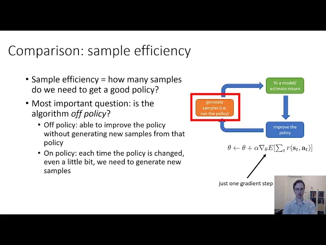
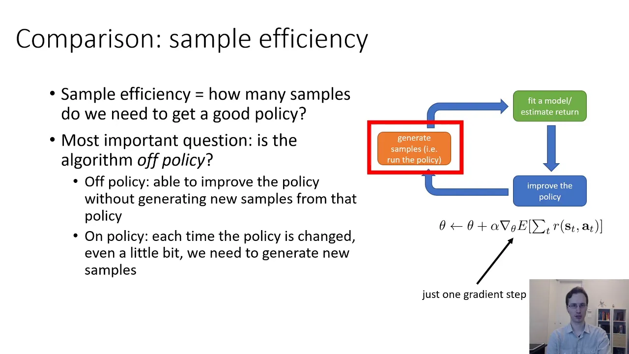
so why do we have so many different rl algorithms why is it that we can't just teach you one rl algorithm uh in a couple lectures and be done with it why do we need an entire course well these are algorithms have a number of trade-offs that will determine which one works best for you in your particular situation so one important trade-off between different algorithms and we'll touch on this as we go through the next few lectures is sample efficiency meaning when you when you execute the stuff in this orange box when you generate samples
in the environment how many samples will you need before you can get a good policy another trade-off is stability and ease of use reinforcement learning algorithms can be quite complex they require trading off a number of different parameters how you collect samples how you explore how you fit your model how you fit your value function how you update your policy each of these trade-offs and each of these choices often introduce additional hyper parameters which can sometimes be difficult to select for your particular problem different methods will also have different assumptions for example do they handle
stochastic environments or can they only handle deterministic environments do they handle continuous states and actions can they only handle discrete actions or can they only handle discrete states do they handle episodic problems meaning problems with a fixed capital t horizon or do they handle infinite horizon problems where t goes to infinity or both and different things are easy or hard in different settings for example in some settings it might be easier to represent a policy even if the physics of the environment are very very complex while in other settings it might be easier to learn
a model than it is to learn the policy directly each of these trade-offs will involve making some set of design choices for instance you might opt for an algorithm that is not very sample efficient for the sake of having something that is easier to use or maybe for the sake of having something that can handle stochastic and partially observed problems or you might opt for a very efficient algorithm because you your samples are very expensive but then be willing to accommodate some other limitations like for example only allowing for discrete actions so typically we have
to make these trade-offs depending on the particular problem that we're facing let's talk about sample efficiency first because that's a pretty big one so sample efficiency refers to how many samples we need to obtain a good policy basically how many times do we have to sample from our policy until we can make it perform well that's the orange box one of the most important questions in determining the sample efficiency of an algorithm is whether the algorithm is what's called an off policy algorithm or not an off policy algorithm is an algorithm that can improve the
policy by using previously collected samples an onpolicy algorithm has to throw out all of its samples each time the policy changes even a little bit and generate new samples for this reason on policy algorithms can be a lot less efficient for instance a policy grading algorithm which is a non-policy algorithm must collect new samples each time it takes a grading step on the policy because each time the policy changes even a little bit new samples must be collected so in general if we uh want to look at a at a kind of spectrum of with
the more efficient algorithms on the left and less sufficient algorithms on the right a major dividing line on the spectrum is whether it's an on policy or an off policy algorithm where on the extreme end of less efficient algorithms will be things like evolutionary or gradient free methods then on policy policy gradient algorithms then actor critic style methods which can be either on policy or off policy then purely off policy methods like q learning then maybe model based dprl methods model based shell rl methods and so on but then we could say well why would
we ever want to use a less efficient algorithm so it seems like we should just go with the stuff on the left end of the spectrum well it's because the other trade-offs uh might not be in our favor as we move to the left for example wall clock time the amount of computation the algorithm needs is not the same as sample efficiency so maybe generating samples for your application is actually very cheap maybe you're using a very very fast simulator for example if you're learning how to play a game like chess simulating chess is very
very fast so most of your computation time will go into updating your value functions models and policies in that case you probably don't care nearly as much about sample efficiency and interestingly enough the wall clock time for these algorithms is often flipped so if your simulation is very cheap you might actually find the stuff on the right end of the spectrum to be computationally less expensive and the stuff on the left side of the spectrum to be computationally much more expensive stability and ease of use when it comes to stability and ease of use we
might ask questions like does our algorithm converge meaning if we run it long enough is it guaranteed to eventually converge to a fixed solution or will it keep oscillating or diverging and if it does converge what does it converge to does it converge to a local optimum of the rl objective or a local optimum of any other well-defined objective and does it converge every time coming from a optimization or supervised learning background you might wonder at this point why is any of this even a question because typically when we deal with supervised learning or kind
of well-defined especially convex optimization methods essentially we only care about nasa converge in reinforcement convergent algorithms are actually a rare luxury and many methods that we use in practice are not guaranteed to converge in general so the reason for this is that reinforcement learning often is not pure gradient descent or pure gradient s sound many reinforcement algorithms are actually fixed point algorithms that only carry convergence guarantees under very simplified tabular discrete state assumptions which often do not hold in practice and in theory the convergence of many of the most popular rl algorithms such as q
learning algorithms is actually an open problem so q learning is a fixed point iteration model based reinforcement learning is a kind of a peculiar case because the model is not actually optimized with respect to the rl objective the model is optimized to be an accurate model the model training itself is convergent but there's no guarantee that getting a better model will actually result in a better reward value policy gradient is gradient descent or technical gradient ascent but also the least efficient of the bunch value function fitting is a fixed point iteration and at best it
minimizes error fit and minimizes what's called bellman error meaning is your value function predicting values accurately but that's not the same as saying does your value function produce a policy with good rewards and at worst value function fitting doesn't even minimize the bellman era or student actually might even diverge many popular dprl value fitting algorithms are not guaranteed to converge to anything in the non-linear case in the case where you use neural networks model based rl the model minimizes error fit which will definitely converge to a good model but there's no guarantee that a good
model will lead to a better policy policy gradient is the only one that actually performs grading ascent on the true objective but as i said it's the least efficient of the punch assumptions one common assumption that many rl algorithms will make is full observability meaning that you have access to states rather than observations or but another way the thing that you're observing satisfies the markov property so no cars driving in front of cheetahs this is generally assumed by most value functional fitting methods it can be mitigated by adding things like recurrence and memory but in
general can be a challenge another common assumption this one is common with policy gradient methods is episodic learning so here's a robot performing episodic learning you can see that it makes a trial then resets and then makes another trial so this ability to reset and try again repeatedly is often assumed by pure policy gradient methods and although it's not technically assumed by most value-based methods they tend to work best when this assumption is satisfied it's also assumed by some model-based sterile algorithms another common assumption very common in model based methods especially is continuity or smoothness
this is assumed by some continuous value function learning methods and it's often assumed by model based rl methods derived from optimal control which really require continuity or smoothness to work well so as we cover various rl algorithms over the next few weeks i'll point out some of these assumptions as we go but keep in mind that many of these methods will differ in the kinds of assumptions they make and also how rigidly these assumptions must be satisfied in order for those methods to work well in practice