over the past year or so we've had a few sph sig events and the discussion around the future of the method has often felt quite interesting and it's touched on high order and the challenges that that poses but there's never particularly seemed like we've had enough time to really go into it in any deeper so i thought it would be a good time to share some of the work i've been doing over the past two years on a new method called lab fm which to some extent bridges a gap between sph and high order finite differences so i'll i'll provide a little motivation and then give um give sort of the detail of of lab fm or the local anisotropic basis function method um then i'll spend some time going through some various aspects of the method so accuracy consistency stability and show some example implementations to highlight its current and potential capabilities then i'll end with a little discussion on the challenges that i think high order mesh-free methods might pose um and i was going to say i'll try and leave a little bit of time for discussion about this but as it's a webinar the discussion will have to be through the q a so i've shown this slide before as motivation for for high order mesh free methods so i mean for any for any given method there are a number of characteristics um accuracy efficiency flexibility with which are desirable and obviously um each method has its strengths and weaknesses so sph in its traditional form has excellent conservation properties and geometric flexibility when we think of simulations of breaking waves and things and it's pretty easy to implement um however the areas that it's let down in are accuracy or consistency so this is an example uh illustration of the convergence properties of you know some typical methods so we've got resolution uh along the along the bottom and that error up the side so with methods like finite differences finite volume finite elements we typically see convergence around second order and we've got high order finite difference methods where we might get convergence fourth sixth eighth tenth order then spectral methods where we where we get exponential convergence but with sph there's typically a range of resolutions where we where we can see convergence typically between first and second order and then after that depending on the circumstances we generally get some kind of plateau where we reach what's often called the discretization error limit i mean high order methods are desirable firstly we want a consistent method because we want to know that as we throw more resources at a problem we're going to get a more accurate answer um but if we have a high order method then we can we can get either a more accurate answer for a given cost or we can get the same accuracy of answer for a reduced cost um and i've been i've been guilty of creating convergence plots like this myself so i think i've probably presented this one at a spheric talk a few years ago and i've taken a few points over a really small range of resolutions less than an order of magnitude i have drawn a nice straight line through some of them and i've just declared that the convergence rate is is 1. 3 but what i've completely ignored is the fact that if i kept on converging my results would get worse um and whilst sbh with convergent characteristics like this still has a raft of uses in many applications it becomes a bit hard to demonstrate that we're competitive with mesh-based methods when these are the convergence plots that we can produce um so we really this really motivated us to think about how we can develop sort of formally high order mesh based methods that that exhibit convergence characteristics more like high order finite differences so i've included this slide called what is sbh because i think the answer depends on your perspective and i think my perspective is a little different to the traditional sph perspective so traditionally we think of sph as a discrete system of lagrangian particles each with a fixed mass and really the density summation becomes sort of the key equation um so from from this equation everything else follows and we get this hamiltonian system where the symmetries in the system mirror the symmetries um in reality and then we get exact conservation of linear and angular momentum and mass and energy now i've spent quite a bit of time working with incompressible and i think this has a slightly different perspective we tend an incompressible sph to start with the navier-stokes equations and instead of building the method from the density summation we tend to construct our numerical scheme around the navier-stokes equations using discrete sph gradient and laplacian operators as building blocks and we sacrifice global conservation for for local accuracy so in an incompressible sbh perspective this equation you know some some sort of sph gradient or derivative operator is sort of the central central element of the method and so really from this perspective sph is just a way of approximating spatial derivatives of some data on on scattered nodes or particles so this work really focuses on [Music] on meta free methods from this perspective um based on sort of generalized form of of this type of operator but we aim to construct it so that so that we get the desired level of accuracy or convergence so before i before i move on to the actual method i'll just briefly briefly run through some of the notation that i'm going to use so firstly everything i show here is going to be in an eulerian scheme with fixed particles or nodes unless i specifically say otherwise um m represents the order of consistency of the method so that is the maximum order of the polymer polynomial for which the method is exact which means our gradient operators should converge with resolution to the power of m and laplacians with resolution to the power of n minus one the stencils they look just like sph stencils um and i'll denote the the characteristic node or particle spacing as s and the characteristic length scale of the stencil is h which is akin to a smoothing length and it's worth noting that the node volumes and masses don't really enter into the formulation at all because this is really based on polynomial interpolation of the data within this stencil so i'll first define this general local discrete operator l on this stencil which is the sum of the differences between the properties of each of the node i and its neighbors multiplied by an i j specific weight so l approximates a a specific partial derivative and this vector of um partial derivatives here and uh kind of flag vector are simply a notation we've introduced to identify which derivative we're trying to approximate so for example if we're trying to approximate d by dx then we set the first element of cd equal to one in which case this term is equal to d by dx so we're saying that we're approximating um d by dx another way of looking at it is that the vector cd contains the desired moments of these weights um wji so the moments being the x y x squared x y um y squared etc for example if we want to approximate a laplacian in an ideal world we'd have the x squared and the y squared moments equal to one and all others equal to zero so i refer to this as a a general discrete operator because it can represent a range of methods so it has the same form as the anti-symmetric sph gradient operator that uh as i've been using in incompressible smooth particle hydrodynamics and in that case the weights wji are just equal to the kernel gradient multiplied by uh by particle volume it could also represent a finite difference operator in which case the weights wji would be linked to the indices of the ordered nodes divided by a measure of the node spacing and this is the operator that we're going to base lab fm around so how do we get a consistent um how do we make that that general discrete operator consistent so first we decide that we're going to construct our ij specific weights from a series of anisotropic basis functions so it's w1 w2 w3 and they're anisotropic in as much as they depend not only on the magnitude of the inter-particle vector like an sbh kernel does but they also depend on the direction of this vector the vector psi is just a series of of coefficients or vector of coefficients and psi is is the vector that we need to find basically so i won't go into the derivation here but the process of constructing the operators is really as follows so for every node we we construct a local matrix um where we introduce the vector of taylor monomials x and for each node we build this matrix which is the sum over the neighbors of the tensor product of the monomials x and the basis functions w so the resulting the resulting matrix essentially each column of that matrix contains the moments of a given one of these basis functions if we then write this linear system any psi which satisfy the this linear system will result in a in a general in the operator l um having polynomial consistency of the order determined by how many elements of these of these vectors we've we've used so we we solve this this linear system and then we use the psi that we get to calculate the weights so if we've set m equals to 6 then in 2d we'll have we'll have matrices that are 27 by 27. we solve those and then we'll find that the operator l has consistency of order six so it's exact for all polynomials um up to sixth order um and that's equivalent to saying that um that the gradient operators will converge at sixth order and the laplacians at fifth order so that's the first part of the method but the key thing really then is how do we choose our anisotropic basis functions so i've explored two approaches um the first is to set the anisotropic basis functions as um a series of the partial derivatives of a radial basis function and that radial basis function could be an sph kernel for instance if we do use an sbh kernel then this has the nice benefit that in the low order limit of m equals one so when we when we just have a two by two system for that uh for that consistency matrix m then we recover the bonnet and lock um sph gradient operators so first order consistent an alternative approach is to set the set the basis functions as the product of a radial basis function which again could be an sph kernel um multiplied by some orthogonal polynomials so hermit polynomials legends or lager polynomials all work similarly well now these these figures in the top and the bottom they show the logarithm of the absolute value of some of these basis functions and we can begin to see what the purpose of these basis functions is so the basis functions split the stencil into regions the higher the order of the basis functions the more the more divisions there are they're effectively sampling the node distribution within the stencil the type based on a radial basis function split the stencil into segments whereas the type based on orthogonal polynomials split split the stencil into um squares or in 3d um cuboids um the conditioning of the matrices that we have to solve these linear systems um to get to get the corrections is dependent on how well these anisotropic basis functions sample the discrete stencil um and what we found is that the orthogonal polynomials give rise to much better conditioned much better condition matrices and they become less sensitive on on the node distribution or changes to the node distribution so it's actually quite simple really that in a nutshell is the local anisotropic basis function method we build consistency correction matrices using some choice of anisotropic basis function we solve them and then we store some weights which we use in a sort of finite difference style discrete operators for our gradients or laplacians so i'll now move on to some numerical results so first we look at convergence when approximating the derivatives of of a function so for our test function we look at um a sort of pseudo-random 16th order polynomial over a unit square um on a node distribution which is disordered and fairly typical of what we'd get in an sph simulate simulation um these these shifts that i've applied to the polynomial or the sort of random part just to just to ensure that there's no symmetries cancelling out any um any errors it's basically to make it a slightly harder challenge for the method so the figure on the left shows the convergence rate um of the gradient as we as we increase the node spacing and on the right we see the convergence rates for the laplacians as we increase as we reduce the node spacing so for the gradients for for orders m equals 2 4 6 8 and 10 we get convergence rates of 2 4 6 8 and 10.
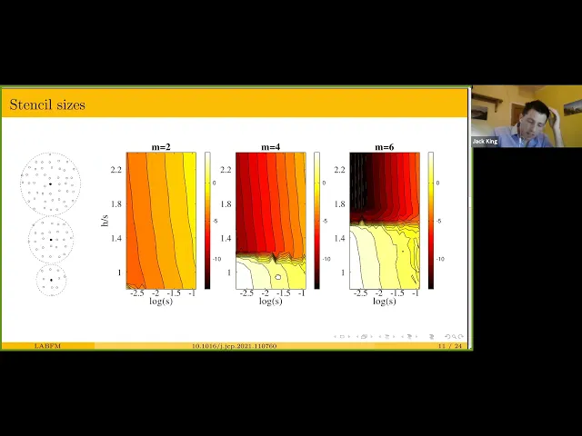
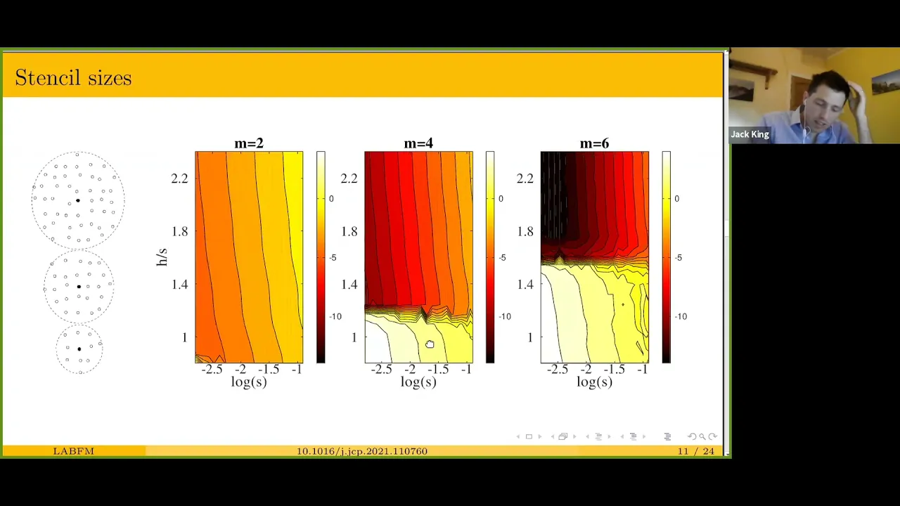
and for laplacians we get convergence rates of one of one three five seven and nine and i think it's worth noting uh these blue lines at the top are the results that we'd get with an sph operator just as standard sbh operators that that i've been commonly using in my incompressible sbh code and you can see that we're getting i've written a fair bit more accurate but really quite a huge improvement in accuracy so in some quite believable circumstances at this kind of resolution we're getting six seven eight orders of magnitude better accuracy um there's still a limiting error um for these operators so for finite difference operators we'd expect convergence rates to continue all the way down to machine precision error limit in in sph the convergence rate is limited by the discretization error which is basically the error due to us not accounting for the particle distribution in lab fm we're accounting for the particle distribution up to a certain order so we get this convergence rate but when we account for the particle distribution we have to solve these linear systems and as we go to higher orders the linear systems get bigger and the residuals from solving them get bigger so really high orders say 10th order then the residuals start to increase and become significant at very fine resolutions so we get this limiting um limiting error levels but they're still an awful lot lower than we call an awful lot more accurate than we could get um with with something like standard sbh so now i'll have a look at uh the effect of changing the stencil size um with lab fm so the color of these plots shows the error with resolution along the bottom and the stencil size up the side so as we move left on one plot we're going to a finer resolution as we move up we're going to a bigger stencil size relative to the node spacing um so we see it's just off the bottom of this plot but we see for each for each value of m so for each order that we're looking at there's a clear limit above which so for larger stencils the method converges uniformly and for smaller stencils the method diverges or certainly doesn't do very well um and this this limit is as i sort of alluded to before this limit is imposed by the requirement that the anisotropic basis functions adequately sample sample the the node distribution within the stencil and if we've got more if we've got higher orders then we have more complex structures in our anisotropic basis functions so we need more nodes in the stencil in order to in order to adequately sample these basis functions it's worth noting that this requirement of stencil size isn't actually that difficult to satisfy so for fourth order um we can get away with stencil sizes of about 20 and 2d or 80 in 3d which is pretty similar to what we'd use in the smooth particle hydrodynamics with with something like a wendland kernel but for sixth order we go up to needing maybe 50 or 60 nodes um in the stencil in 2d and if we were to go to 8th or 10th or 12th order then we'd end up needing sort of 100 odd nodes in the stencil the next aspect of the method i wanted to look at is is the resilience to the to the re to the node disorder so the plots are similar to uh to the ones on the previous slide but here as we move upwards we're going from a uniform distribution of nodes to a severely disordered distribution of nodes um and again we see that these vertical contours indicate that the convergence rate um is is pretty uniform up to really quite high levels of of node disorder so for for fourth order we can get up to almost almost um node disorder of the same order as the node spacing for sixth order or eighth order that drops a bit but ultimately a node disorder of 0. 5 corresponds to a distribution which looks a bit like this which is worse or sort of more disordered than we're likely to get in in an sph type simulation um so it looks good it looks like we can we can have simulations where the accuracy remains high even when we have quite severely disordered nodes or particle distributions so i'll now move on to to some actual fluid dynamic simulations so i've implemented lab fm to solve the the isothermal compressible navier-stokes equations and in most of the simulations i show the spatial discretization is is sixth order um time integration is with a third order runge-kutta scheme the code's written in fortran and parallelized with mpi plus openmp and we employ um sort of high order filtering or de-aliasing technique to stabilize it now there's there's really no two ways about it high-order co-located methods require some kind of stabilization um in spectral methods they they use a d aliasing by just eliminating the top third of the spectrum um in finite differences they often use filters so we we construct a lab fm based high order filter where the coefficients are set in some pre-processing step so they satisfy some the aliasing rule and we use this to stabilize the simulation so it's it's very very closely comparable with with the approach that's used in high order finite differences um by way of a brief validation um on the right there are two figures um i'm just going to close the window because it's raining heavily on the right there there are two figures um showing the error when simulating taylor green vortices um so there's an analytic solution for taylor green vortices in the incompressible limit um but our our simulations are isothermally compressible so in the top i'm using sixth order lab fm and i'm um i'm reducing the compressibility and i see that as i reduce the compressibility we we keep between fifth and sixth order convergence but we we lower this compressibility uh related error limit on the bottom i'm keeping the compressibility fixed um but changing the order of lab fm from fourth sixth eighth to tenth um and again at ten eighth and tenth order we we encounter this compressibility related error limit um which is just an unavoidable consequence of comparing this compressible simulation with with an incompressible analytical solution but above that limit we get well order of between three and four between um five and six between seven and eight and between nine and ten convergence um which is very nice so i also i've pointed out here that this is eulerian but although it's a rather slow simulation to conduct i've also conducted this test with a lagrangian plus particle shifting ale scheme and with that framework where i have the particle positions updated with the with the third order runner cutter scheme along with the velocities and density logarithm the convergence plots are unchanged so the results are almost identical and they would be identical when you look at them in the view of these plots um which is a nice feature because it shows that if we can have a good lagrangian particle updating scheme then we can get very accurate results um with the lagrangian mesh3 method so taylor green vortices are periodic and it's really a comparatively easy problem uh boundaries they present a more significant challenge um and that's because so whilst partially filled stencils like this one on the left are okay um we we can get up get away with up to the penultimate row of nodes um at fourth order and so the third from the edge row of nodes at sixth order however if we go all the way to the boundary then even at fourth order um these stencils aren't okay actually they're okay in terms of accuracy but they're not okay in terms of stability um and the filtering technique that we have at the boundaries can't handle the the high wave number noise that these stencils would introduce so here's where we combine with with finite differences so on the boundaries we use a strip of nodes um with a in a sort of ordered regular distribution um with fourth order one-sided finite difference stencils and with these one-sided operators that allows us to use um a characteristic based boundary formulation which is particularly nice because then the numerical boundaries that we implement can be can be imposed in a way which is consistent with the physics of the problem so we can use this for arbitrary geometries but the caveat here is that we need to resolve the curvature of the geometries um so if we have a geometry with some very very fine curves in it then we need a very small resolution another nice benefit of these boundary conditions is that we don't have the additional computational and memory overheads of storing an extra set of ghost or mirror or dummy nodes or particles as we often have to in sph so that this boundary framework is quite attractive because it doesn't it doesn't increase the cost anymore by having these extra nodes so on the bottom of this slide i've got two examples the first on the left is of a lam ocean vortex passing out of the domain on the right um with negligible distortion to the vorticity so it's just a demonstration that this this boundary framework combining lab fm plus finite differences allows for for very nice accurate um non-reflecting outflows um the second one is this video which which shows flow past the cylinder and again we can see the um we can see the pressure field and the vorticity um propagating out through the right hand well through the through the outflow with negligible um distortion and also although it's not visible in this in this image any um any pressure disturbances moving upstream are nicely propagated out of the the non-reflecting uh inflow boundary condition so briefly i'll just show a small amount more validation so we've compared the results um with some experimental um some published experimental data so this is it flow past and impulsively started cylinder and we match we match the experimental data quite well so we we have the center of the vortices uh in the same position we get the stagnation point matching and we also get the formation and position and size of these little secondary vortices matched quite nicely on the right we've got a comparison with spectral element methods so this is looking at the steady flow behind the cylinder and when we look at the velocity profiles in these transects um behind the cylinder um we get an extremely good match uh with published um spectral element methods um which is it's just a nice little for the sort of confidence booster that that our code is doing the right thing so so far i've not mentioned variable resolution um but that's not because lab fm is unable to handle it actually it's because it's not an issue so the only real requirement is that we remember to adjust the node spacing s and the stencil size h in tandem and provided we'd do that and it works fine so both of these stencils this uniform distribution and this sort of spatially varying distribution both of those are fine um and on the right we we i've got the the convergence plots for the gradients on a on non-uniform distribution and you can see that we again we're getting um second fourth sixth eighth and tenth order convergence all the way down to the to similar error levels um even with this uh this non-uniform node distribution this video the bottom highlights the kind of node distributions that we can then generate so this is this is flow past um past an ellipse and i'll just go back to the start and you can see that we've got really quite a significant range of resolutions um i think it's by a factor of about 80 over the domain between the smallest and the largest um and really we don't have to do anything special to handle this this change in resolution we just have to make sure that we adjust the smoothing length um h and the node spacing in tandem um i wanted to also mention here that the flow can handle quite so the the solver can handle quite challenging flows so this is transonic flow pasta pasta ellipse um the color here shows the the local mach number which is is quite quite significantly above one in certain regions and so we can capture the the generation of shocks as vortices are shed off the ellipse and i think at the second half of this video it'll show um that we can capture the acoustic noise generated um so yeah this this is showing the acoustic noise generated by this vortex shedding and we see these little shocks um propagating around the ellipse i'll just skip to that again so so the method's hand capable of handling sort of incipient shocks without too much dissipation so a final example that i wanted to show is a more complex geometry um this is a representative porous matrix and discretization again is is fairly trivial um so i've only just learned how to do videos like this which is why you've got a lot of zooming in videos but you can see again that we can we have our band of finite difference nodes around the around the porous around the solid boundaries and then we have a smoothly varying resolution um varying again by about two orders of magnitude and between the smallest and the largest um so this video shows that the method can handle can handle this type of flow for for low mach numbers so this is a mach number of about 0. 15 a poor reynolds number of just below 1000 and we can see the velocity field as more and more vortices are formed in the downstream section of the of the porous media this figure this video on the right shows a slightly more challenging case so we've we've increased the poor reynolds number to 2000 and increased the the poor mach number um the inflow of the of the of the forest media to uh not 0.
8 um so we've got maximum local mach numbers of of about 2.