[Music] foreign [Music] hello everyone and welcome back today we're going to continue our exploration of multiple linear regression and consider two mechanisms that can be used in order to detect which variables in a multiple linear regression model should be kept or should be removed based on its contribution to our model so let's just go over a few Basics that you definitely need to understand in order to work through these two concepts which are known as the partial f-test and partial correlation coefficients so we of course start with a multiple linear regression model let's assume it has the structure Y is equal to beta0 plus beta 1 x 1 plus beta 2 x 2 all the way down to say beta p x p plus our residual Epsilon so in this particular picture we have p predictor variables all right so usually what we do is we try to see is this model with these predictors X1 X2 down through XP are they good predictors for this variable y so the null hypothesis h0 that we typically work with is that these coefficients beta 1 beta 2 all the way down to Beta B of course The Intercept is not one of them all of them are equal to zero with the alternative the beta I is not equal to zero for at least one I so that is our null and alternative hypothesis that we typically work with so a couple statistical metrics that we use to test this are first off the MSM which is equal to the sum of squared errors for our model divided by the number of predictors P which can be found by SST minus the sum of squared residuals all divided by P and keep in mind SST is just the variance of our response variables y times the degrees of freedom M minus 1 for those y values and then we also have our MSE metric which is just going to be equal to the error sum of squares the sum of squares residuals divided by n minus P minus one and if you don't remember how to find your SSE you can always calculate the sum from J is equal to 1 to n of your observed y values minus your predicted y values and then Square each of those residual differences all right that's going to give your SSE and of course you divide that by n minus P minus one so from these two statistical metrics we build what is called an F's test F test statistic which is given by fstat which is equal to MSM all divided by MSE and as long as the normality assumption and independent assumptions are met for our multiple linear regression model then both MSM and MSE will follow a chi-square distribution hence the quotient will follow an F distribution and in particular we'll follow an F distribution with p m minus P minus one degrees of freedom and obviously since we're working with the alternative that at least one of them is not equal to zero and this test statistic based on its structure and its direction because typically MSM is usually greater than or equal to MSE not always but most of the time as long as we have evidence for rejection therefore this will be a right-tailed test therefore if this is your F distribution this is where your Alpha is located and obviously with that Alpha is associated a f critical value and then we can compare that F critical value to that F test statistic and then decide whether we reject or fail to reject this particular null hypothesis so let's briefly outline what that conclusion looks like so if the associated p-value because from a test statistic we can calculate a p-value if that Associated p-value is less than our Alpha value and then we will reject the null hypothesis and that beta 1 equals beta 2 is equal to Beta p is equal to zero which means what which means that at least at least or all of our model coefficients all of our model coefficients appear to have appear to have a good contribution contribution to our model right and if the p-value is greater than alpha or you could say greater than or equal to Alpha then we will fail to reject this null hypothesis that beta 1 is equal to Beta 2. is equal to Beta p is equal to zero which means at least one of these coefficients is equal to zero right in particular the null hypothesis says that all of our coefficients are equal to zero um but it's possible that one of those coefficients are so close to zero that is pretty much weighing down um the other coefficients in our model so if at least one of these coefficients is equal to zero or moreover if all of those coefficients are equal to zero one can ask the following question so if some values of our beta let's call it beta case R close to zero is our model better without them so that is the question that the partial f-test seeks to answer let's start off with a numerical example to sort of guide where this discussion is going to go so let's assume that we have a multiple linear regression model with three predictors X1 X2 and X3 as we already know beta hat which is represented by X TX inverse xdy where X is the design Matrix the First Column of ones the rest is our data values for observed values of X1 X2 and X3 y are observed value vector and sigma squared the Hamas elasticity variance which we should be able to approximate with the MSE since that's the none biased estimator so with these two things that we know already let's assume that these are the values in green so beta hat zero negative 36. 7 uh standard error for beta has 0 13.
5 obviously those are usually larger but that's not the concern for the um good contribution of our predictor conversation right so our focus is primarily with our beta hat one two and three so usually what we are looking for is predictor slope values I. E these beta hats that are really close to zero obviously if all of these values are close to zero then we're going to be failing to reject that null hypothesis that all of them are equal to zero but if this or if the least value is significantly close to zero in this case 0. 52 will probably be the most closest of the three then it's possible if that's really close to zero depending on the unit and the standard error then it's still possible that we will be failing to reject the null hypothesis even though our other variables are at least on the surface contributing to our story so if that is the case enter in our beta hat 3 is the closest to zero a natural question that we can ask is do we keep our predictor X3 right now it's very very important keep this in the back of our mind X1 X2 down to XP could be in different units right so for example beta hat one could be an age Beta had two could be in terms of height Beta had three could be in terms of weight but what exactly are the units for these beta hats so let's actually take a look at our model so if Y is equal to Beta 0 plus say beta1 X1 plus beta 2 x 2 plus beta 3x3 plus Epsilon and let's assume that our variables are X1 X2 and X3 and obviously that means Y is a variable two and we take the partial derivative of y with respect to one of our X's say let's say x j then that's obviously going to be equal to Beta J so the unit on beta J will be that of the partial derivative of y with respect to X so that's obviously this beta J in terms of its representation is a unit change in our x j results in a beta J change in y right so if you change XJ a lot and your beta J is close to zero that means it's not contributing to the story at all right so that's how we interpret these particular things and obviously so if we take for example X1 to be equal to age X2 to be equal to height and X3 to be equal to weight then these beta coefficients are for example and let's assume we're trying to predict happiness in that Vector y then we have for example happiness over age happiness over height happiness overweight and obviously since they have different units we should not be comparing them in their original form so it's possible that 0.
52 actually is not close to zero with respect to the other two because they would have different variances in different variance units Associated to them right so there are a couple approaches that people use um so I'll present both of them to you so approach one to fix this issue is to standardize or what people call standardizing the coefficients standardize the coefficients so what we do keep in mind beta hat J is already in the unit unit of Y all over the unit of X so if we can somehow cancel this unit of Y from the top and the unit of X on the bottom then we have a metric that doesn't have any units so what we can do is we can define a new metric I'm going to call it beta hat J with a superscript s for standardized beta hatch a this is going to be equal to our beta hat J from before that had the unit but on the top we're going to be multiplying by the standard deviation of that random variable and the standard deviation of Y on the bottom because when we multiply by this the unit on the bottom is y that's going to cancel at the top and the unit on top is the unit of x j which is going to cancel with the unit of x j on the bottom and therefore this has no units so that has no units so that's one way you can look at the new coefficients and compare these so we can compare different units because if we use the beta hat JS then they're not going to have any unit so it's fair to compare now all this although this does fix the issue it's usually not the more preferred way especially if you plan to get other features for your model that is a little bit more advantageous obviously this fixes one way but it's just fixes one thing in order for us to compare so let me introduce another approach which I find more appropriate and instead of standardizing the coefficients we standardize the entire model and this actually gives us several advantages which I'm not going to discuss here so what we're going to do is we're going to Define variable ZJ to be equal to the variable XJ minus the mean of those x j values all over the standard deviation of those x j values so therefore keep in mind before we had for example Y is equal to X beta in terms of our Matrix representation which is again beta 0 plus beta 1 x 1 all the way down to Beta p x p so what we're doing is we're taking our X values we're subtracting the means of those observed X values and dividing by the standard deviation so if x is normal then this random variable is technically a t random variable right right so these coefficients beta hat One beta had two beta hat p are all going to change because our variables are going to change because this has no unit it has no unit so when we standardize our variables then we're going to have a new model our new model keep in mind we're not changing y here so we're going to have for example y now instead of beta0 we're going to have a new variable I'm going to call it Zeta zero and then we're going to have Zeta 1 Z1 plus Zeta two Z2 all the way down to Zeta p z p plus the standardized version of our residual let's call it Zeta Epsilon right so there are P standardized variables and here we have the coefficients of our standardized model so these are our coefficients of our standardized model which should not to be confused with the standardized coefficients where we just focus on the coefficients only right now you will get the same predictions from each of these approaches because technically you're not really changing the model in the first one but if you use this model you're actually going to have the same p-value the same f-stat um uh same r squared same r squared adjusted value so you're not losing anything but you have a different model in particular one of the things that change are these coefficients and they will not have any units and just as a side note these units are these coefficients are not the same as the standardized coefficients mentioned in approach one so keep that in the back of your mind so this is still a multiple linear regression model so you still can solve this with the usual approach so obviously we're going to approximate our Zetas with Zeta hats so our Zeta hats is going to be equal to z t z transpose z t y right so that is going to be the solution and keep in mind these Zeta hats do not have any unit so let's you know use the same numbers that we had before so keep in mind we had for example beta hat one which was 26. 3 beta hat two which was equal to minus 13. 5 and beta hat 3 which is equal to 0.
52 if you forget that these actually have any units it's very easy to say oh I probably want to throw out beta hat three but you shouldn't because they could be in different units so we standardized these coefficients and obviously we had a beta hat zero but we don't really care about it but it does turn into a new Zeta hat zero which is again going to be different but that's not our Focus and we're going to have for example a Zeta hat one which is like 2. 61 you're going to have a Zeta Hat 2 which is negative 1. 32 and Zeta hat three which is equal to 1.
83 now one important thing that's actually pretty interesting to sort of think about is the signs of our coefficients both in the original and are standardized predictor model will be the same sign just different values right so if it was a positive before it's going to be positive again if it was negative before it's going to be negative again but these do not have any units now here you would look for the smallest value in terms of magnitude in this case that would be Zeta hat two So based on this criteria alone you probably would vote off variable two if you were to vote off something based only on this criteria so now let's go back to our original model which was beta 0 beta 1 x 1 beta 2 x 2 all the way down to Beta p x v plus Epsilon from here on we're going to be referring to this model as our full model up to this point we have a or possibly multiple criteria for deciding for deciding which variables to remove so let's assume that we're at that stage of the story where we decide to eliminate e predictors here e is going to be a variable it's not the 2. 71828 number I don't have that many letters to work with so let's just call E to be the number of eliminated predictors from our model so what is the most or the highest value that e can be so let's actually subscript these uh beta ones uh with something in particular I'm going to call this beta 1 F beta 2 F down to Beta p f and Epsilon F to represent my full uh predictors right because I don't have to choose these predictors I can choose any subset of them right so in this case I have p f predictors and my full model so the maximum number of predictors I should be able to take away obviously you should not be taking away all of them because then you're just going to be left with the lonely little intercept therefore you don't really have a model if you take away PF minus one that gives this simple linear regression model and if you're removing something obviously the number of removals should be bigger than one so from this logic we see that one must be less than or equal to e must be less than or equal to the number of predictors we're removing from that particular model all right so e is the number of eliminated predictors right so if that is the case the number of predictors so let's do a little before an after chart number of predictors so before we had for example p f predictors and we're going to be removing e of them so we're going to have p f minus E which we're going to Define as PR and PR is going to be the number of predictors in our reduced model all right so when we have our reduced model what exactly does that model look like well obviously our response variable is y is not going to change so we're going to have y is equal to Alpha 0 plus alpha 1 x 1 R plus Alpha 2 x 2 R all the way down to Alpha p r x p r right so this is our oh let's not forget our little Epsilon term at the very end so these are our remaining e predictors right which is a subset of the original right so for example if we started off with seven this model might have five might have four might have two it might have one right it might have six but I can't have seven right it has to have at least one less than it used to have and it has to have at least one so from this set obviously I've renamed my coefficients Alphas instead of betas because they're not going to be the same exact coefficients because you know we're going to have you know possibly emitted variable bias right because if we remove variables from our original model and those betas were not equal to zero then those beta values are going to sort of spill out into these new Alpha values in our reduced model so how are we going to calculate these Alphas well that's still a multiple linear regression model so we can still use the same um biased estimator for those outputs so for example Alpha hat is going to be equal to x t x inverse but these are the reduced design matrices X and then Arc xrt why so from this new set of beta hats in some sense then we're going to have for example A reduced SSE A reduced SSM and an SST but keep in mind this SST is the same as before right so for example SSE plus SSM always is equal to SST but sser and SSM are are pop most likely different especially if those values are non-zero in whatever variables that we actually removed so what's going to happen to our SSE is it bigger than before is it smaller than before what exactly is going on there so as long as the removed let's call them xjs weren't identically identically identically identically zero then we will have what so as long as our SSE is greater than zero which we typically assume that it is else we have no variance to model then which is going to be bigger SSE r or ssef or ssef is the full SOC that we started with you might want to take this video and pause it for a moment and think about this on your own before I type the answer but the full SSE model is going to be less than or equal to the reduced SSE model and obviously those are always bigger than or less than or equal to SST so we always have this relationship which means the SSE is going to increase when we remove predictors but that obviously is going to lead to emitted variable bias because as I already mentioned those beta hat values are going to spill into those Alpha values and you know you're not going to see as much of a distinguishable effect in this particular predictors right so you have this particular relationship right so we're increasing um those sses but hopefully we're doing it for a good reason so let's take a look at what the Anova table uh for this reduced model actually looks like so a Nova table for our reduced model so obviously we have our error source and our degrees of freedom are sum of squares and our mean square error right so we have since we're working just with one set of variables we're just going to have one set of residuals we have the error for our model and then obviously we have the total error and our model so our degrees of freedom for our total is not going to change that's still going to be remaining at n minus 1. for our reduced number of predictors that's going to be equal to the original number of predictors PF minus the number of variables that we removed and then for our degrees of freedom for our residuals that's going to be n minus P minus 1 which in terms of our original is equal to n minus the original number of predictors plus the number of variables we've reduced minus one and if you're not sure why it's a plus because technically there is a minus sign before we distribute that into the parentheses so what I want to do is actually just write that as a minus and put a parenthesis next to it or you can just remove the parentheses and distribute the negative and make it minus PF plus e minus 1 depends on your preference and comfortability right but that is are your degrees of freedom for each of these entities and that should be M minus 1 of course so once we have our SOS obviously we can calculate our mean squares but again this is going to be our SSE reduced and you calculate the same exact way but you have different residuals now you have our SSM R and you have your same SST so usually we calculate our SST or sscr and we can calculate SSM by subtracting or it could calculate it directly if you want really no matter there and lastly once you have your sses and you have your degrees of freedom just divide your degrees of freedom into your sum of squares and you can get your mean square error so you're going to have for example a mean square error for your reduced Model A mean Square uh error for your model for the reduced model and then you're going to Simply have your MST which is still your SST over M minus 1.
so once you have your imported metrics MSE and MSM then you can calculate your F statistic so fstat is going to have the same structure which is going to be your MSM all over MSE but this is of course for your reduced model and this will as usual follow an f p f minus E comma n minus p f plus e minus 1 distribution and is still a right-tailed test and as usual the null hypothesis is that Alpha One equals Alpha two all the way is equal to Alpha p r are all equal to zero now hopefully you have a p-value that is not close to zero or farther from zero as before because keep in mind what we're trying to show here when we're removing these models is that this model is better than it used to be which means we're trying to reject that null hypothesis right because our null hypothesis is that Alpha One is equal to Alpha 2 is equal to all the way down to Alpha PR is equal to zero so our goal is to reject if this is truly better so if our goal is to reject then that p-value should be smaller if I misspoke before I'm sorry for that but the p-value should be smaller than it used to be if it's not then you sort of haven't really gained anything from that but even if we do have a p-value that is smaller than before for example let's assume we had a p-value of I don't know let's say 0. 07 for a full model and let's assume we have a p-value reduced of 0. 03 obviously if you have an alpha value of 0.
05 that's going to be a better difference you probably will be happy but if this is our result then we have more evidence to reject this null hypothesis which may imply to you that this model is better than before but technically no because keep in mind we are not considering the other predictors that we remove removed in this hypothesis test they are independent tests so it doesn't directly answer that this model is better than before but it can in some sense tell you whether this model is good or not for predicting the value of y independent of what predictors you removed so let's quickly address that and clarify that if need be so what we have up to this point is two models the full model and the reduced model so we decide which predictors we want to remove from our full model and then we can have these two independent hypotheses tests or testing the equality of our coefficients to zero right so for example let us assume um that we fail to reject the first null hypothesis about the betas so if we fail to reject the null hypothesis for our betas um then that means either one or many of these predictors are close to zero obviously in the first example that I illustrate it it's possible that one is very close to zero and is dragging all the others down so if that is the case then you probably would want to remove variables if one or more betas are close to zero right because if we remove those things that are close to zero then most quote unquote are going to be not far from zero anymore because we removed all the ones that are far from zero of course this leads to a minute variable bias but sometimes you can address that indirectly with other Advanced methods right so that is one scenario where you would uh look into this but of course it's possible that we would reject the null hypothesis that all of our betas are close to zero right which means we have evidence to believe that all of our betas are far from zero then in this case you probably would still want to consider removing predictors to make our model better right obviously they're not far from zero but we want them farther from zero maybe right so there's two different scenarios of where you might want to consider removing protectors now as I've already mentioned the analysis see the analysis of null hypothesis beta is equal to the zero vector Alpha is equal to zero Vector these do null hypotheses are independent of one another right so one does not affect the other at least not directly right so if we're using this particular model it does not answer the question is the model with Alphas better than the model with betas in it so that is the next question that I want to answer so question how to test the question is model Alpha better than model beta that is we're comparing directly these two models so one way you can do this is what is called a partial so I'm not going to go through the derivation of these particular things but I will give you the F statistic and we can briefly talk about this so the partial F statistic which I'm going to call PF stat is going to be equal to SSE R minus SSE full keep in mind SSC full is always going to be smaller than or equal to SSE R so this difference is always going to be positive all over n minus PR minus 1 minus n minus p f minus 1. so what exactly does this term focus on so we're seeing has our SSE significantly changed so that's what this is pretty much looking at and we're going to be dividing this by our SSE full because that's going to make it bigger than one and that's going to be divided by n minus p f minus 1. obviously there is some simplification that can be done here for example if we look at this piece right here we're going to have n minus PR minus 1 minus n plus p f plus one uh our ends are going to cancel with one another our ones will cancel with one another and this is just going to be equal to p f minus PR which we know is just the number of variables that we eliminated so we can actually represent this partial F statistic as the following so PF stat can be equal to or represented as SSE R minus ssef all over e where e is the number of eliminated variables divided by ssef All Over N minus p f minus 1.
right so that's a nice little way to write it and you could also rewrite this in another way but again it really depends on what you prefer and what you're more comfortable with you can write this as n minus p f minus 1 over e so that's just our coefficient times our sser minus ssef all over SSE f right I think that's a more nicer way of understanding sort of what's going on here and this as long as our assumptions are met that both of them follow the normality assumption Independence this is going to follow an f e n minus p f minus 1 distribution and as usual that would be a right-tailed test so this test statistic once you calculate your F statistic in the associated p-value this is going to be testing the null hypothesis that there is no significant difference between our models with the alternative is that m a m alpha is statistically different is statistically different then our model for our betas right which is usually what you want to do if you're trying to show that one is better or worse depending on what other conclusions you got from the above analysis right but this is how to test whether this model is significantly different from each other because for example if your P value just goes from 0. 7 to 0. 6 some people will say Ah that's not really that much different right 0.
5 to 0. 4 0. 3 to 0.
2 0. 1 to 0. 10 right they are close right so this is going to help you decide whether there is a statistically uh statistical difference between them before moving into the last thing that I want to mention I just want to remind you of a couple correlation coefficients and coefficients of determinations that are commonly used in multiple linear regression just in case we don't already know what they are one of them is called of course the multiple multiple correlation coefficient which is just going to be the square root of the coefficient of determination some people just use the r squared value some prefer to use just the R value and some people also note this as y given a particular value of x and this can be calculated via the square root of 1 minus SSE all over SST right so that is our multiple correlation coefficient and r squared the multiple coefficient of determination r squared always being between 0 and 1 and R always be in between negative one and one and what this tells you is the strength of the linear relationship of Y and a particular value of x right but keep in mind we're in multiple linear regression worlds so this x is actually a vector so if I don't want to write this in an ambiguous way one should actually write this as y given a particular value of X1 X2 down to XP where X is the number of predictors so that's a particular random variable and then we have another useful metric which is called the adjusted multiple correlation coefficient and the only reason this exists is because as you increase the number of predictors the SSE will go to zero inherently as long as you're not introducing uh just a bunch of zero predictor vectors but the adjusted multiple correlation coefficient tries to counteract that by changing the SSE over SST into MSE over MST so the adjustable multiple correlation coefficient is of course going to be the square root of the multiple coefficient of determination AKA r squared adjusted which is sometimes just abbreviated as just r adj and as far as I know there's not a subscript for random variables but I guess you could still subscript this with Y given X1 X2 down to XP of course the notation gets a little messy but you know nonetheless it's implied there and that's just going to be equal to the square root of 1 minus here MSE all over your MST now this is not often used at least uh from my understanding because the r squared adjusted value can be negative and since we're taking the square root of a potentially negative number it's possible that this might not exist because you can't take squares or negative numbers in the real plane but you can always take the magnitude of that complex number and compare it to zero still but it really depends on what you're going for right and also some people will use the notation r y given X as just the correlation between Y and all of your variables or technically you could say this is going to be equal to the correlation of Y with your predicted variables now what if you want to ask the question or answer sub questions rather is there a good correlation between y and a subset of variables with potentially canceling out the interaction of of the remove of the removed variables with the variables I'm interested in analyzing so let's take a look at what that looks like so this is called a partial correlation a partial correlation so let's sort of let's just actually just write this down so suppose we want to know the correlation between y and X1 but other variables for example say X2 might be influencing might be influencing the relation between Y and X1 so is it possible to sort of remove the interaction of X2 with Y and X1 and sort of just have y and X1 alone even though in some sense they probably are mixed together else why would we be doing a multiple linear regression model between them so this partial correlation coefficient is going to be noted as r let's do it Y and X1 with X2 held constant so this is the partial correlation just the partial correlation with or let's say of Y with X1 with X2 let's say partialed out or phased out I guess it's a more appropriate word so this is going to be calculated in a very interesting way and you can sort of think about what's going on here if you have some theoretical understanding of the formulas this is going to be the correlation between Y and X1 so that's just a bivariate correlation coefficient so that's just you know Y and another variable this is not a multiple correlation coefficient but you can extend that if you want to sort of know the correlation between y X1 X2 with X3 phase out or something like that so that's going to be equal to minus r x1x2 actually here's a better way I think let's do y with X2 and then our X2 X1 I think if I write it this way and you want to explore this on your own this representation might give you a little bit of insight and that's going to be divided by the square root of 1 minus r let's see here what do we got going on I think possibly a more safer way to write this is to keep in the same order as the top so let's just write it as y x 2 and then square that put that in Brackets and then 1 minus r x 2 x 1 squared because our rx1x2 and rx2x1 is the same exact thing so that is a commutative so this gives us um the partial correlation of Y with X1 with X2 phased out of the picture right so what exactly does that look like on our analytical viewpoint so if we have y is equal to beta0 plus beta 1 x 1 plus beta 2 x 2 plus Epsilon and let's assume we're trying to remove this like we want to sort of phase that out but maybe we don't have the time to run another multiple linear regression model maybe we can figure out huh can we analyze what will happen between Y and X1 if we were to construct a multiple linear regression model because if Y and X2 do have a strong linear relationship maybe we shouldn't remove X2 and if Y and X1 have a strong relationship almost like to 1 if it's an r squared value maybe we should remove beta 2 because there's not much room to sort of contribute or maybe they're the same exact dependent variable or something like that so one very interesting theorem is the following if we consider the SSE removed minus SSE full divided by SSE full this particular quantity but this is precisely equal to the r squared value for the model y X1 with respect to X2 being removed so let's put that square on the outside of that parenthesis right so that's the partial correlation coefficient partial correlation coefficient so that's interesting so in some sense they have a connection so if that is the case then you can actually calculate your partial F test statistic in the following way because this bracket should look familiar so this is actually equivalent to doing the r squared value for y X1 with X2 phased out squared times n minus PF minus 1 all over the number of variables that we've removed now keep in mind if X2 really is a variable then e is just equal to 1.
but if X2 is a sequence of random variables for example X2 could be in Disguise you know beta 1 or beta 4 x 4 plus beta 5 x 5 plus beta 7x7 where we're considering you know removing four five and seven and we're sort of phasing that out from the rest of the model then in that case e would be equal to 3.