Graph Convolutional Networks (GCN) | GNN Paper Explained

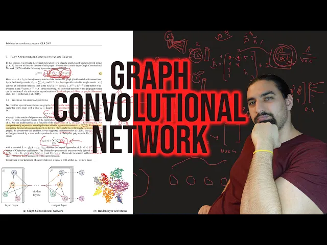
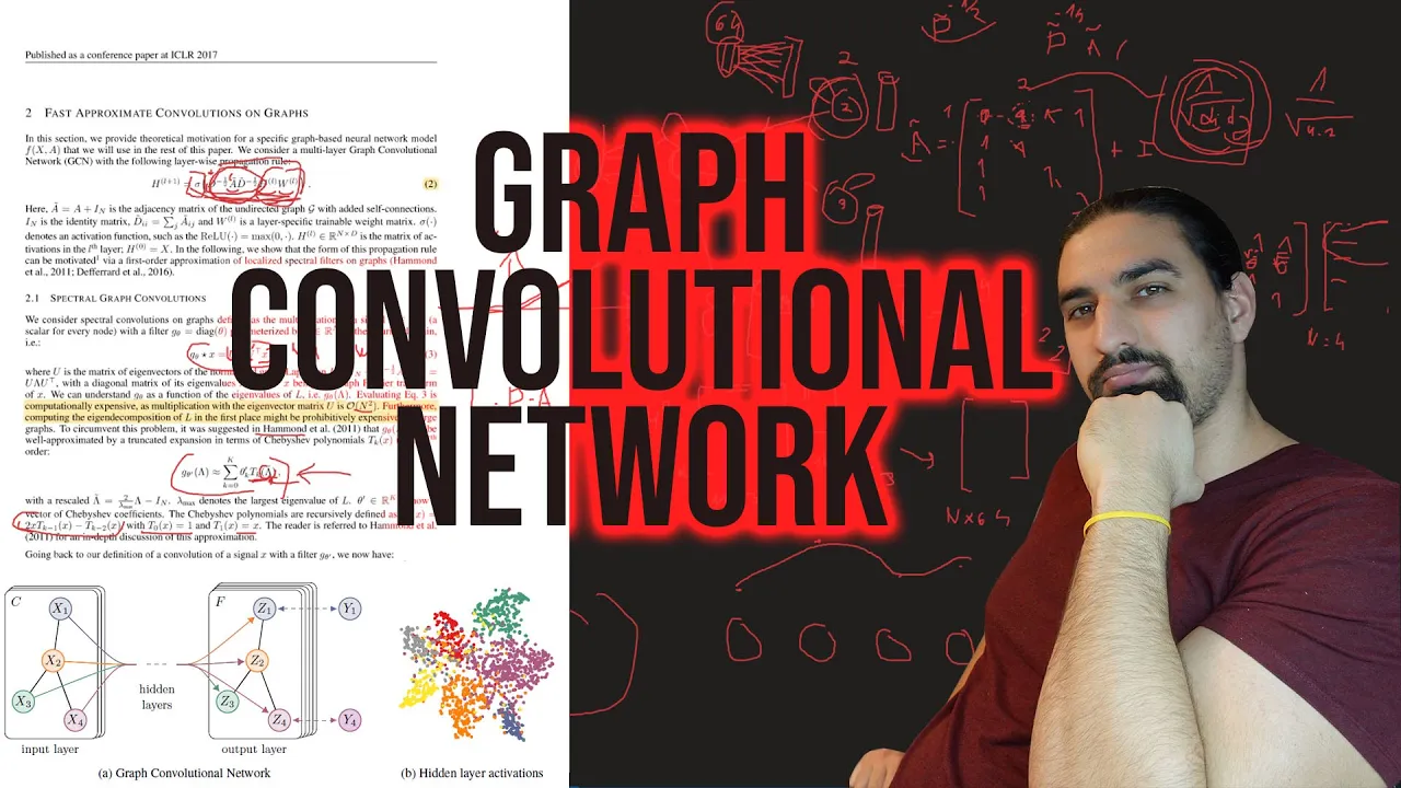
what's up uh in this video i'm continuing with the series on graph neural networks and i'm going to cover the semi-supervised classification with graph convolutional networks or gcns for short that's the most cited paper in the gnn literature and it was published by thomas kipp and max welling so basically this paper can be uh looked at from three different perspectives so the one they uh they they they showed here in the beginning of the paper which i'll briefly explain uh is the spectral uh so just considering their method as a special case uh as an

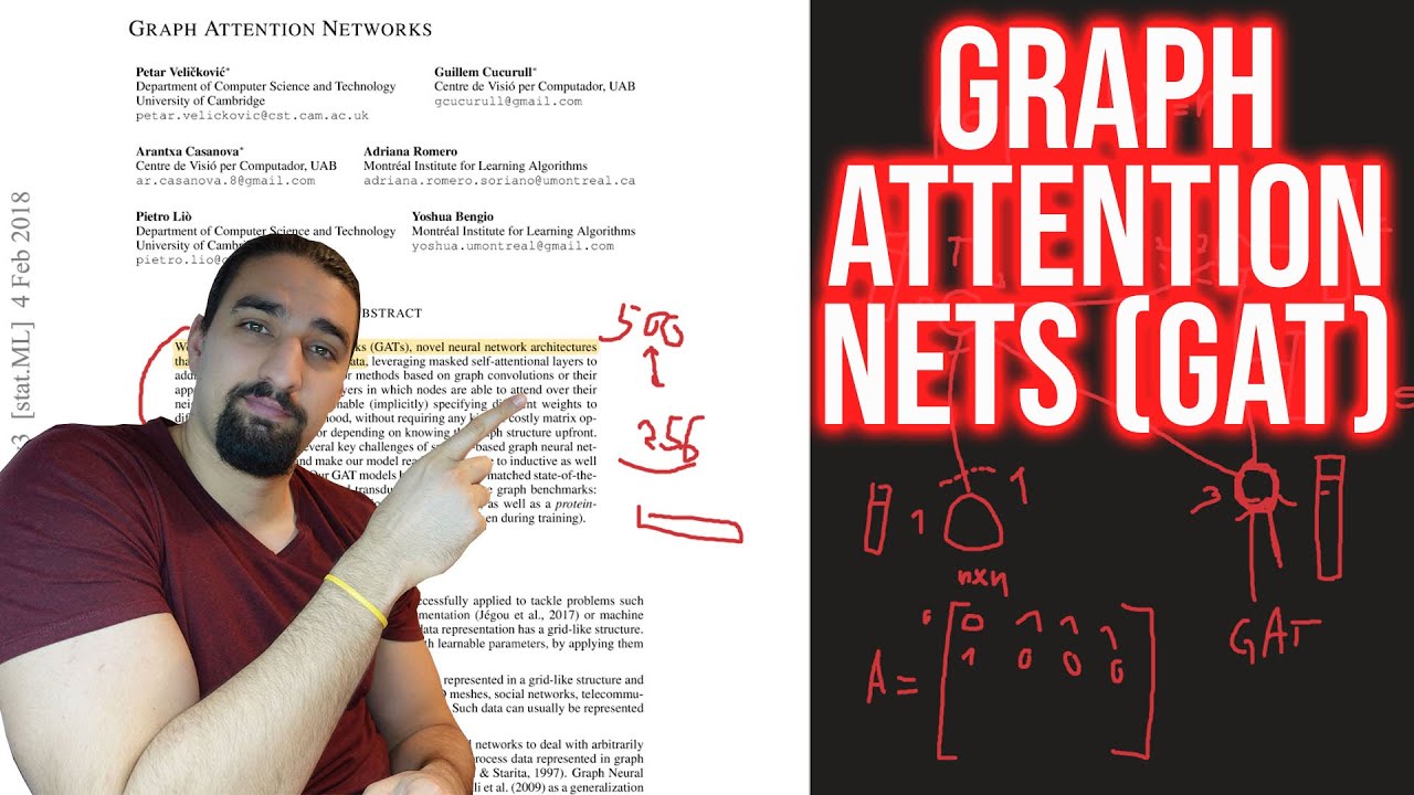
approximation to spectral graph methods the second perspective you can take is considering this is a generalized vice ver layman algorithm and the third approach is basically just treating this as a as a specific case of a message passing neural network or like maybe even a get graph attention network which was the paper i covered in my last video um so i'm just going to before before i jump into the like explaining the method and the the spectral uh perspective i'm going to just tell you about uh these uh explicit uh graph location regularization methods so

uh previously before gcn came and those spectral methods came uh we mostly had like two classes of algorithms we have on we had on one side the graph embedding algorithms such as deepwalk such as planetoid et cetera and on the other side we had these methods that did a semi-supervised learning using these explicit graph locations so let me just uh show you what this regularization uh term uh does so basically if you take a look at the the semi supervised uh loss here we have the supervised portion the the l0 and we have this regularization

so and you can see here how it looks like so basically what it does is it enforces the nodes which are connected to have the same label or similar labels so it just smoothens out the labels and that's just a hypothesis uh that's just a prior the bias this method has it wants to make that the locally connected nodes have the same label which is something that not that might not be a good thing to do in all in all the problems but sometimes may be a good idea as well so they say here the

formulation of equation one relies on the assumption that connected nodes in the graph are likely to share the same label this assumption however might restrict modeling capacity as graph edges need not necessarily encode no similarity but could contain additional information so gcns showed later we'll see the results that they outperformed all of these baselines and it's much better idea to just let the the neural network learn from the features and from the graph structure then by just uh encoding this uh this bias into the model so what what this uh thing does and i'm going

to draw a simple graph here because we'll need the adjacency matrices and all the terminology later so let me just draw a simple toy graph here and do some simple connections like this and this may be node number one node number two three and finally four so how the adjacency matrix looks like is the following so that's an important concept and i'm going to repeat it even though i covered in my last video uh so basically um what it does it it just represents the the the the connection pattern of the graph so we have

zero here because node zero node one doesn't connect itself it doesn't have a self connection and we have once here because it connects to all of the other nodes and the other nodes just connect to node number one so we'll have ones here and we'll have zeros elsewhere so basically uh now what this equation does here is you just iterate through this adjacency matrix and you take the corresponding labels and you just uh subtract them and you square them so basically that means if we go through the row number number one uh we'll we'll basically

have uh we'll take we'll take uh this one and let's say for the sake of argument this one has uh the label two uh node one has label one node three has maybe label three and this one also has label two so what we'll do here is we'll take because we have uh so this is node number one this is node number two we have one here so that means it will get included into this sum and we'll just take the label so the label from this node is 2 so we take 2 we subtract

1 and we square it up and we repeat that the same procedure for wherever we we have one or wherever we have a connection in the adjacency matrix so basically we'll have uh label three here we'll take three minus one and we'll square it up and again we'll have 2 here minus 1 and we'll square it up and we can see that none of these goes to 0 and that's what this graph location regularization term enforces the method to do so in order for this to get to zero all of these labels should be uh

changed to to to to basically uh two to one because that's what this node has so that's it in a nutshell uh so again f is just a function that maps the feature vectors that are associated with every node and just gives us the class and we want those to be uh similar and smooth so basically this this regularization term won't allow it the method to to assign label 10 for example to node number three uh if you assume we have ten classes so that's it in a nutshell so now i'm going to cover i'm

going to first cover how the the gcm works because um it's it's better to have a mental picture a clear mental picture of how it works before we go into the motivational like the the spectral perspective so this is how the the the equation to how the how the gcm works so we have this constant term which won't change um during uh the propagation because it contains the adjacency matrix with it add itself connections which is the tilde term here uh the tilde symbol and then we have the green matrices which also contain self connections

and those are just raised to the power of minus one half uh which i'll briefly like i'll explain what that means in a sec and then we have uh h which is just uh like a matrix of feature vectors for every single node and we have w which is just uh the linear projection layer and again for the sake of easier understanding uh this part i'll just uh i'll just draw this this graph so i'll take the same example as before so we have a graph we have some connections like this one and now what

we do is the following so we again have the matrix adjacency matrix a and uh so we had like uh the pattern was like this we had uh ones here because uh node one connects to both nodes two three and four hence the ones here and then we have ones here because node number two connects only two to node number one and we have zeros elsewhere so now um to in order to make this uh like the tilde version we just need to add an identity matrix here which basically just adds the self connection so

we'll have ones here we'll have ones here we'll have ones along the diagonal pretty much and what this does is basically assumes we have self connections on every single node so once we have this matrix a tilde we need to normalize it and we do that by doing by using these uh degree tilde minus one-half terms so what does uh this represent what does this mean uh basically this degree tilde matrix just does the summation row wise along this a tilde matrix so we'll have a diagonal matrix which contains four here because we when we

sum up we'll get four uh four here and that's that what it means is basically this is a degree we have four connections going to this node number one that's why we have four here then we have two two and two because all the other nodes have uh only two connections okay so uh the next step is just to inverse it and do a square root so basically what we end up doing once we once we multiply the d tilde raised to the minus one half times a tilde and we do the same thing here

we basically uh normalize all of these ones with this term with 1 over square root of d i times d j now what d i means is it's basically the degree of a node i and d j is a degree of node j so basically this particular node which now has one corresponds to so that's a connection between node one and node two right so that's this connection and because this node has degree of two that's the dj and this one has degree four will basically just normalize this term so this one here with one

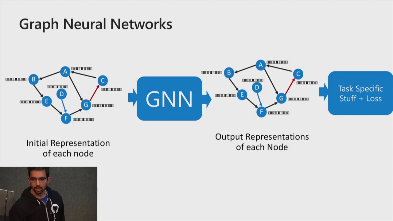
over square root four times two and that's square root of eight whatever that is so that's what we do and that's how we normalize this matrix and now all of this will uh hopefully fit together in a moment so i just wanted to explain uh how that matrix is calculated so so how the process looks like in the gcm method is the following so all of these nodes have associated a feature vector and for the sake of being less abstract let me say this one has 1433 features and for example this number is not like

random quora data set the citation network which this paper also used as a benchmark has this many features per node where every node represents a paper in a citation graph so basically all of these nodes will have this feature vector and high level what the method does is it first projects these uh these feature vectors using this matrix w which we can see here projects projects them into some lower usually lower dimensional space so it will basically be a fully connected feed forward layer without the activation at this point or you can just treat it

as an identity activation which is the same thing and so basically this one will maybe have 64 dimensions and once we do this for every single node in the graph we end up having so that's this part and now what this part does and i'll explain why it basically just accumulates or aggregates which is a term used in the graph literature these features and it just scales them using these square root over di dj things and you add them up and you get the the new representation so basically uh this vec this node 1 will

accumulate all of the vectors because all of them connect all of these nodes connect to it so it will have so its final representation will contain some portions of all of these other feature vectors on the other hand if we take node two uh it will have only the feature vector uh that came from itself and that came from node one so that's the difference so you just basically take the one hop neighborhood you just aggregate those projected features you sum them up but before you you sum you use those like uh sk these scaling

factors and that's it you basically only apply after you do that you apply some non-linear differentiable activation functions uh such as value and i assume everybody knows what really is but i'm gonna just draw it for the sake of argument so basically it's an it's a like a zero here and uh pretty much uh y equals to x uh in this part so if you still can't uh associate this equation with the process i just described i'm going to go once more and explaining the exact process that goes on in this vectorized form so what

i i want to explain concepts i try and do it as intuitive as possible but like uh these all these equations are usually vectorized and which makes them uh less maybe less intuitive but once you kind of get the hang of it it becomes really easy so let me try and explain every single matrix so h matrix is basically as i said you just we just stack horizontally all of these future vectors so because we have n nodes this h matrix in the zeroth level so initially it will just be uh basically n times whatever

the dimension here is and that's we said a thousand four hundred thirty three so this one will be so again it will be n times one thousand four hundred thirty three that's the size then we have this w matrix and w projects from 1433 into we said i took like as an example i took 64. so it will be a matrix that has the same dimension here will be here so we'll have pretty much 1433 times 64. so it will have 64 dimensions here so basically this corresponds to this one and once you multiply these

matrices so h times uh w will end up with the new matrix which which contains the projected feature vectors for every single vector for every single node in the in the in the graph so we'll end up with a new matrix some intermediate matrix that has a dimension n times this time 64. and those are these small vectors i draw here and here etc so hopefully that part is so far so good so that's this part okay and finally we need to multiply by this by this normal by this um normalized uh adjacency matrix and

let's let's figure out that part so now we have so let me take this example we already have concrete numbers here i just don't have uh these one over di dj parts but you can just imagine they are there and what we do so i'm going to redraw it again here just to make it a bit more clear so we have ones here we have ones here and because of the self connections we have once along the diagonal as well everything else is zero so uh i just stack four nodes because n equals to four

here right in our small graph we have only four nodes so we stack up those 64 uh dimensional vectors and i won't draw every single element because they are initially some random values so basically uh what we do is the following so the first node as you can see because it has all ones it will basically take into account every single projected vector and that's what i previously explained so because it's connected to everything it will take all of the feature vectors uh the projected ones and it will just uh uh add them up and

we have those terms as i mentioned which i want uh whatever like square root whatever corresponds to the degrees of those notes so uh that's that's the case for the node one but let's take for example nodes two so node two only have has one here and one here and it has zeros here that means once you multiply this arrow with this matrix you'll just basically take these two feature vectors and that corresponds to the thing i mentioned previously and that's just you just take this feature vector and you just take this feature vector and

you add them up and you use those uh scales again and that's that's why the equation works and it basically does the same thing as what i just intuitively explained here using the drawing hopefully this uh this makes sense and i went into a lot of details uh please let me know if this was too too detailed painfully detailed or it was just right so i appreciate the feedback now the reason they use uh these uh coefficients here to to to normalize the adjacency matrix values is because if we didn't do that we'd have a

problem with exploding or vanishing gradients which can nicely be seen through this spectral prism which i'm going to explain right now so basically if you're familiar with eigen decompositions uh what those sk scaling coefficients do is basically they make sure that the largest eigenvalue of our matrix is equal to one so basically they make sure that the range of eigenvalues is between zero and one and by just continually applying that matrix we won't have um exploding or vanishing gradients so that's that's that's the trick so this part by just constantly uh multiplying by this term

if the eigenvalue range is in a good in a good range basically we won't have the problem i just mentioned with vanishing or exploding gradients so because the the spectral part is really complicated it deserves a video for itself i'm just going to briefly explain the main ideas here and uh hopefully uh if you think that that could be useful i'll cover the the spec some of the spectral methods uh in one of the next videos although they are not as popular as these spatial methods where gcn is one representative get is another representative etc

graph sage etc so how it works how the the spectral graph convolutional method works in a nutshell is the following so you take the laplacian matrix which is basically a degree matrix and you subtract the adjacency matrix and you find the eigen decomposition of this matrix and you get eigenvectors and you get eigenvalues so once you stack up those eigenvectors in a matrix you get these u matrices and what you do is you take the signal on your graph x so what's the signal so just for the just for the sake of being of being

uh clear um so basically you take these feature vectors you take maybe first feature from every single feature vector and you can treat those as as a signal so basically imagine we have we we just align these nodes linearly and we take those first features from all of the feature vectors and maybe this one has a value like this maybe this one has a bit bigger value and you basically can treat this if i interpolate some random interpolation you can treat it as a signal a discretized signal on the graph so what we do here

in the spectral method is we project that signal into the uh into the new basis defined by the location eigenvectors and those are contained in u then we have this this is what is learned in these methods so we don't learn the w matrix as previously in gcn we'll learn this filter g data g sub data and now the problem with this is and it says here it's computationally expensive as multiplication with the eigenvector matrix is o and and so we go notation and square so basically uh because this matrix u is m times n

and x is uh n times one because we remember we just took the like first feature or whatever like just one feature instead of the whole uh feature fully blown x matrix which has all of the features so basically that's why we have a computational cost of n squared and that's not the only problem the second problem is that doing the eigen decomposition of the location is super expensive it's i think it depends on the like uh there are more optimal methods depending uh on certain uh like uh details but like oh of ends and

a cubed is probably a good estimate of the complexity and so that's super expensive so then there were so hammond uh and his collaborators suggested that we can just uh instead of learning all of the n parameters here so where n is the side of the graph which can be in the size of billions if we're doing dealing with for example facebook graph or pinterest wherever and basically you can we can treat this we can just compute like a uh like a k polynomial and using using chebyshev polynomial and we can just uh use this

approximation now i won't get into details how this approximation came to be that would be a separate video but like just trust me on this one and it can be shown that instead of using so this matrix here lambda contains eigenvalues we can ditch computing the eigen decomposition and we can save those n cubed computations and we can just do a chebyshev polynomial using the this the slope plation matrix instead instead of using the eigenvalues matrix so chebyshev you can see a simple recursion again won't get into much details it's really simple recursion we start

with one and x and this is how you combine them to get the next uh polynomial terms and you basically end up having so this is how we do uh convolution spectral convolution now so we just have k terms here we have k parameters so these are scalars we just learned these and it's much more efficient this time so the thing with this uh this equation here approximation is that it's in contrast to the pure spectral methods like this one this one is k localized and that means that pretty much means that all of the

if we have a graph and you take a single node it will only capture the features from its k-hop neighborhood so meaning um the the the neighbors which are further away are only our arcade edges uh far far off from from this target node so uh why this is because um if you know something about adjacency matrix properties if you just raise it to the power of k what you end up doing is the term i j in this matrix will tell you how many uh paths there are between nodes i and j uh like

k length bets so basically um that's that that's the reason why why uh why we have a k-hop neighborhood here um now again you if you didn't understand this detail it's totally fine um that's not the point of this video so now what gcn does is basically it starts from this approximation so this is an approximation of the fully blown spectrum method and it it it does the following it just says let's just treat uh let's just take a look at one hop neighborhoods we don't care about k-hop neighborhoods we want to make set k

to one so no so as they say here now imagine we we limited the the layer of ice convolutional operation to k1 so that's the first approximation they do and so they say it here nicely we intuitively expect that such a model can alleviate the problem of overfitting on local neighborhood structures for graphs with very wide node degree distributions such as social networks citation networks knowledge graphs and many other real-world graph data sets so that's the explanation the the argument why they set k21 uh basically for certain graphs like citation networks which they are using

uh as benchmarks in this paper like cora sites here etc uh they can be um they are basically uh something called small world networks and this approximation makes sense the second approximation they do is they say here we further approximate lambda max so the the the maximum eigenvalue to be approximately two as we can expect that neural network parameters will adapt to this change in scale during training okay so basically once you take those so k equals to one and lambda max equals to two uh you basically going from this equation you end up with

uh with this one and uh basically now you can just uh um if you take a look at what while lambda uh why why l minus identity here is because they are using uh they are having a chebyshev polynomial of uh this scaled laplatian so basically what that means is so if we expand this polynomial we'll end up with first term will be i the second one will be this uh l tilde then we'll have um two l tilde squared minus i etc uh depending how many how big the k is so if we if

we consider l max to be two we'll ditch this term and we'll end up with uh l minus identity and that's what we get here so that's the l minus identity part and now finally uh there is uh one more approximation they do and that's uh constraining these two to be the same thing so theta zero and theta one let's read them uh to be the same parameter and you can extract it and basically you get this equation and the the last trick they do because if you take a look at this matrix the range

of eigenvalues will be uh from zero to two which means if we continually keep on multiplying features x uh projected features we have theta here uh times this matrix will end up increasing the values or the consequently the gradients will either explode or diminish and that's something we want to avoid and that's why they do this normalization trick and what they basically do is they add up self connections and we saw that when i was explaining the method itself uh so basically that's it once you once you uh just uh swap this part with this

part you end up with the final method and that's the the form i previously i previously explained um so the good thing about this method it it has a complexity that's proportional to the number of edges in the graph and not to do like uh a number of nodes uh like raised to the power of three uh for like uh spectral spectral methods which was super super uh compute intensive so yeah it was a it was a mouthful there is a lot of details and you need to read a couple of papers to understand every

single part so for example why this approximation works um why we can where we can swap uh eigenvalues with locations here and um yeah that's probably the hardest part then you can just this is simple thing uh this one is also conceptually simple and a couple of more steps and you're we're at the final stage but that's why i said uh that maybe uh uh not looking at uh at the gcn through this spectral prism but by looking at gcn maybe as a special case of get method or as a message passing uh network uh

in general is much more like feels more natural than than treating it as a spatial as a spectral method because it's not spectral method we don't have to compute it's not like the final expression doesn't have to do anything with spectrum we don't have to compare to compute eigenvalues you don't have to compute eigenvectors so it was just motivated by by the spectral methods but it's not a spectral method itself so just avoid being confused there the hardest part we covered the method we covered how i was motivated by the spectral methods and we saw

how the uh the explicit graph uh laplacian regularization works so now let me just walk you through the rest of the paper a couple of more things details so once you pre-trained gcn with two layers on the quora data set and you extract the hidden layers the hidden features you can project them into 2d space using t-sne and you get this and if you remember if you if you watch my previous video on get you can see that uh get maybe had a a bit better separation between quora classes than gcn but once you actually

uh once you and you can you can also verify that because it had had better accuracy uh than gcn but i'll get to those results in a bit but basically um you can you can see that get actually has on these types of networks on citation networks the attention coefficients it used for the neighborhood are pretty similar and kind of approximate gcn although it's more more expressive and thus has a better results okay so again semi-supervised learning uh pretty simpler simple thing and i explained that in get but like for the sake of being uh

complete here uh you just do cross-entropy so you basically have a huge network and you just take for every single class and quora has like seven classes you only take 20 notes whose labels you're going to use you don't use other labels you you do use the features but you don't use the labels and finally once you get to the final layer um the the feature vectors now have the number of classes uh like seven for quora and you'll just do you'll just do cross entropy loss on on those on those on those values and

that's how you train uh these models so basically for the sake of being clear um so what what we do again let's say this is quora so we start with 1433 we do the projection we do the aggregation so in the hidden layer we'll have maybe 64 features and again we do apply another layer and because cora has seven classes the final feature vectors will only have seven uh features and we do soft max so we end up with a probability distribution and we just take a look where the true class is and we do

the cross entropy so if it's maybe 0.4 the loss will be log 0.4 and just a minus there and that means this needs to go to 1 for the ground truth class in order for the loss to go to 0 which makes sense and you just do gradient uh based learning and they used atom for gcn and that's it in a nutshell and again they visualize these features here let's see a couple more things uh in this paper uh the next thing is so i already mentioned we have uh previously to gcn and the spectral

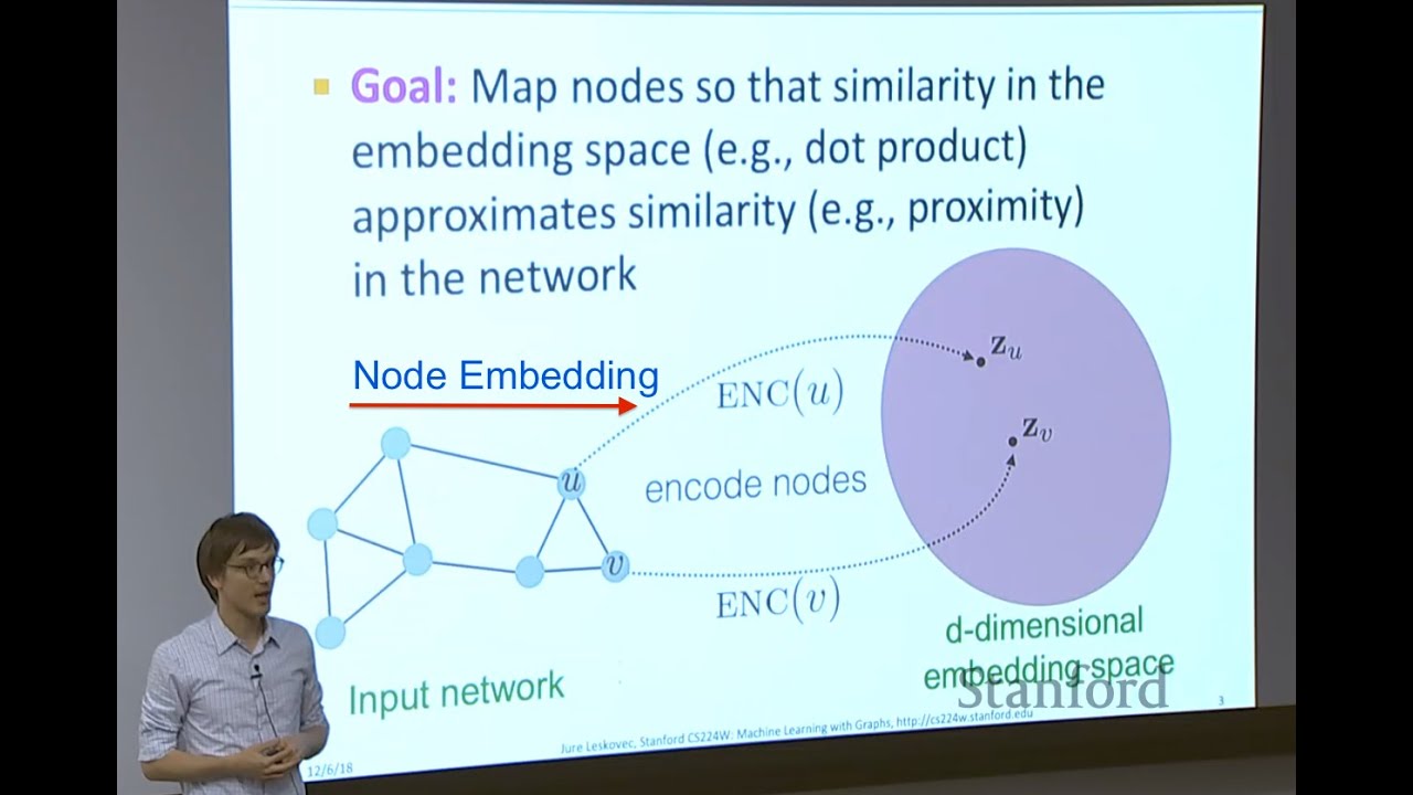
methods we have we had two broad categories the ones that use explicit graph location and the one that used a graph embedding approach so the graph embedding approach basically creates random walks it's similar to vertovac if you're familiar with nlp um yeah it's basically the same idea just applied to graphs you treat uh random works on graphs as sentences and you basically train your embeddings such that they are uh such that uh the ones that appear uh close to each other tend to have similar embeddings in a nutshell um so i mentioned previously uh they

used three citation networks sites here core and pubmed they use this knowledge graph as benchmarks and yeah i mentioned that quora has thousands so this we were using this example as a as a as on the fly example throughout this video and basically you can see some statistics related to that uh like uh data set and it has seven classes as i already mentioned so um and i mentioned they're using only 20 labels per class so so that means so you have so you have uh the core has 2 700 nodes but you only use

440 uh to train the the the gcn method okay they also have some random graphs i'll explain those briefly why they mentioned those ones okay so um here are the results you can basically they compared against these these methods used at explicit graph location regularization deep walk and planetoid or graph embedding methods and here is gcn and we can see on every single data set they have a significant improvement compared to the baselines and uh yeah that's uh nice okay uh finally they compared uh different methods and this is the reason i had to go

into a bit more details in the spectral uh section part uh so basically they compare the chebyshev so the one uh the the the the approximation of the full spectral method and they tried using k2 and k3 so that means they're using k uh two hop and three hop neighborhoods and you can see the results are worse than gcm method and the renormalization trick is the official the final gcm method you can see uh so here going from top to bottom are the approximation we were making so here uh we just set k to one

uh then we we we constrained these two thetas to be the same here in the single parameter uh row and we can see that all of the results are worse than by using the final uh the final dcm version they also compared against the first order term only so they ditch uh this part and they just use the the first order term and we also get verse results and finally the reason i highlighted mlp here is that it doesn't use the graph structure and you can see that the the performance the the accuracy is far

like lower than all of the other methods so that's the reason so even so so basically it's really important to use the the the graph structure because it contains a lot of information so how they trained mlp i suppose is so again you have you have the graph and you have features associated with them and you just basically independently apply the mlp here so this is maybe the first layer and then you have the second layer and you end up with seven classes here and you just take those 440 nodes sorry to to basically train

this mlp and you basically repeat the same so these are the same weights these are the shared weights you apply them to the first uh feature vector then you go to the second one blah blah blah you apply the the the cross entropy loss and you train the mlp and that's and that's so so you can see in this process it's not using the connectivity pattern so it's ignoring the connectivity pattern all together okay let's continue and finish up wrap up this paper um there are a couple more things i want to mention the first

thing is uh and this is interesting so so basically um you can see the training times here on the y-axis we have seconds per epoch and on the x-axis we have number of edges and this is where those random graphs can come into place so what they did is they just create uh n uh notes and they just take two n edges and they randomly uniformly just connect all of these uh notes and that's the graphs they were using and they just use a futureless approach where basically you just have a one hot vector or

the adjacency matrix is pretty much the identity matrix and they use these graphs to just a benchmark like that to test the speed of these of their models and we can see that uh as we go to a huge number of edges the speed is still around 1 to 10 seconds on cpu and gpu and compare that to transformers which need days upon days of like huge machines to train them and but once you think about it it's not that interesting because we only have a w matrix in the case of gcn to train and

that's a small number of parameters although as the number of nodes gets bigger the computation also gets bigger but using sparse dense matrix multiplication and some methods you can you can speed it up but it's interesting it's really it's really fast to train these networks and that's that's cool okay let's go and see a couple more things so i mentioned uh memory requirement and so i'm actually currently implementing the graph attention um network and i'll open source it in a couple of weeks probably uh but like the the hardest part i found uh like implementing

these networks is how to uh uh efficiently implement the the layer and that's that's pretty much everything because you you wanna there is all of these like sparse uh formats and mages uh sparse dance matrix multiplication is happening and how what's the best way to represent your edges whether using edge index or just using the plain old sparse adjacency matrix and then finding some suitable format to represent it anyways i don't want to get into too much detail just keep that in mind that pretty much the hardest part here uh is to like efficiently implement

these methods um yeah they see here our framework currently does not naturally support edge features and is limited to undirected graphs weighted or unweighted uh that's that's something to keep in mind because both quora and all of these uh benchmarks they used they don't have any edge features they just have like simple binary connections okay that was the the main part of paper i mentioned uh in the beginning of this video that i have three perspectives we can treat this so we can we can look at this gcn paper through three different perspectives the one

is spectral method perspective and now let me show you the second one device file layman algorithm so basically uh wl algorithm or vice versa lemon specifically the 1d case of this algorithm what it does it's an it's a simple isomorphism graph isomorphism test what that means is basically you have two two graphs so graph g1 and you take second graph graph g2 and you pass it in into this test and it uh if the if the final uh something called node colorings are the same no if they're different then you're most you're sure that these

two graphs are not isomorphic if they're the same you're still not completely sure because there are special special cases where uh vice volume like fails but like you're pretty certain that uh those two graphs are isomorphic and what isomorphic means is basically you you those are just two same graphs but just have different maybe different labeling and if you find some different like permutation of labels you can see that those two graphs are the same and there are some really nice examples i'll show it here on the screen and you can see those two graphs

are are the same even though they look differently uh like at the first glance so that's the idea with device fileman algorithm and now you can treat gcn as a pretty much uh as a generalized version of of uh of this vice valemian algorithm and with the disclaimer ll in a couple of seconds explain why that's not completely true but let's for the sake of argument now let's play the game uh so this is how the algorithm looks like so we start with initial node coloring and you can treat maybe this uh the same as

so we have those features the same as we used so far and basically the algorithm stops once those uh features stabilize and it's basically the same structure so we have repeat until it's basically going through the layers of our gcn and we for every single node what we do is we aggregate the features or the colorings in this in this case that we aggregate them and we hash them and that's what's what our updated representation looks like and if you think about it it's really similar to what we have with gcn so basically we aggregate

across the neighborhood again and we have these cijs which i've mentioned a lot of times already and that equals to one over square root d i d j where those are degrees of those particular nodes and if you take a look at it it's the same format you can treat just the hash part is maybe the non-linearity and these projections and scaling but it's it has a similar structure and they say here this loosely speaking and it's really important to to highlight the loosely speaking part because it's not completely true and and you'll see in

a minute uh allows us to interpret our gcn model as a differentiable and parametrized generalization of the one-dimensional vice versa algorithm on graphs and now the disclaimer so basically uh later uh this paper called graph isomorphism networks uh appeared and it showed that gcn is not quite there so they say here this is just a snippet from the paper so we we will see that these gnn variants get confused by surprisingly simple graphs and are less powerful than the wl device volume test nonetheless models with mean aggregators like gcn perform well for node classification tasks

and we used exactly the node classification uh benchmarks in in this paper so this paper used those benchmarks so that's why uh we couldn't know this i mean this paper appeared only later so it was hard for them to to compare but um anyways they showed that these gene uh gin networks are more expressive uh than gcns and more expressive that gets also so that's something to keep in mind i won't get into too much details but basically there are certain uh families of graphs which uh if you if you input them so you have

graph one and you have graph 2 and they are different but once you pass them into gcn it would give it will give them the same note coloring which means gcn treats these two graphs the same like they are isomorphic but they're not they're different so gcn can fail on some on certain uh graph families as well as get uh but yeah that's something i thought it's worth mentioning just to keep connecting uh those dots across different papers uh finally so i mentioned the third perspective get perspective so basically you can treat the gcn as

a particular case of get where you have instead of learning those weights you just have them uh hardcoded uh as this expression which i've mentioned multiple times already so that's about uh that's it uh and finally uh is a nice consequence of of of this of the fact that you can treat this as a wl algorithm uh so they say here from the analogy with the wl we can understand that even an untrained gcm model with random weights can serve as powerful feature extractor for nodes in a graph so what we do here we just

take these w matrices and we leave them we leave them like a random and basically so this a hat is the term with uh d tilde mine raised to the power of minus one half etc so just the constant term so we just apply uh three layers here uh three adjacent layers and this is what we end up with so we have this showed here that if we take this karate club network so if you take this network and you just take a features approach meaning all of these nodes don't have some meaningful features they're

just like the adjacency matrix is pretty much identity matrix and if you pass it through the untrained gcn it will still learn how to separate uh different classes so what it did is so basically the last layer of this gcn has only two so the the node features have only two dimensions and thus they can easily be plotted on a 2d chart like here and you can see that clusters like this one which have the same labels also appear in the same part of the space in this 2d space here so that's interesting that means

that gcn can without any training already have some discriminative power just because of the graph structure and finally uh once you start training uh this gcn the through layer gcn i just mentioned you can see it gets even better separation and finally after 300 iterations the classes are clearly separated and that's that's awesome uh one more last thing is uh experimenting with depth so if you if you think about it all of the networks gcns i mentioned so far i had either two or three layers so what's up what's up with that you know if

you if you're familiar with computer vision you know that cnns usually have a bunch of layers like resnets had i had 151 or more layers and basically here we'll use two or three so what's what's the thing so basically they they showed here that uh and they've uh added these skip connections basically uh uh just adding the the representations from the previous layer uh like this and this is the original equation so using these models they showed that uh after two or three uh layers we get to peak performance on the test and we don't

need anything to go any further so and that's that's interesting and uh the the the explanation here uh you can you can search for it uh michael bronstein had a really nice blog wrote a nice blog about this and i'll just quickly summarize it so basically since grids are special graphs there certainly are examples of graphs on which depth helps it's just a quote from his blog and what that means is that pretty much you can treat image as a as a grid as a regular graph and we know that for images depth helps so

that means there are certain classes of graphs where depth does help but here on these citation and knowledge graph graphs for some reason depth doesn't help and one of the explanation that michael gave here is that one of the differences is that the lat ladder are similar to small world networks with low diameter where one can reach any node from any other node in a few hops so you probably heard about this facebook graph where at least i heard about it i'm not sure if the numbers are truly correct but like you can you can

get to any single person on the graph on the facebook graph by just in like six or seven hops so that means that the diameter of the of the facebook graph is around seven i'm not sure if that's entirely correct but you get the point so it's so intricately connected that already after a couple of players you've basically touched a lot of the neighborhoods neighborhood neighboring nodes and you don't need any more layers to to achieve better performance so that pretty much wraps it up uh hopefully you found this video useful um i'm experimenting i'm

i'm i'm still figuring this out so if you have any feedback for me i really appreciate it i'll continue uh creating gnn videos throughout january and if you have any any requests please write them down in the comments section i'll try and and maybe create some video depending on what you folks uh like suggest me if you like this video and if you found this channel useful please consider subscribing and click the bell icon to get notified when i upload a new video so that you can get my videos as soon as they get uploaded

and until next time keep learning deep [Music]