This is my machine and for some reason it's learning what's up code Squad if you're new here welcome to the squad and if not welcome back my name is Kylie ying and today I'm going to be talking about machine learning more specifically we'll dive into supervised learning and then we'll learn how to use tensorflow to create a neural net and then use a neural net for some text classification sound exciting let's get Get started all right jumping straight into things the first thing that we're going to do is go to cab. research. google.com and it'll
pull up a page like this you're going to click new notebook this is going to create a new notebook and let's retitle this to free code cam tutorial okay it doesn't really matter you know what you actually um rename it to As Long as You have a notebook open And just in case you know you have some future notebooks that's why you want to rename all of them so the typical libraries that I'll import when I usually start a computer data science project are numpy so import numpy as NT pandas import pandas as PD and
then import map plot lib Okay so because I'm going to be using tensorflow in this video I'm also going to import tensorflow as TF and then import Tensorflow Hub as Hub okay now if you click shift enter it'll run this cell another thing that you can do is click this little play button over here that will also run the cell so cool yeah if we click that that runs the cell as well all right so the first thing that we're going to need to do before we can actually do any data analysis is upload a
data file so this little folder over here this is where we manage our data or sorry this is where We manage our files and I'm just going to drag and drop the CSV file the link is in the description below into here so click okay and you'll see that this is currently being uploaded sweet might take a while because this is a pretty big data set we can wait until this yellow thing goes all the way around all right so pause all right sweet now wine reviews. CSV has uploaded to this folder which Means that
we have access to it in this notebook now so now what we can actually do is import that tsv file as a data frame using pandas which is this Library here that we imported so what I'm going to do is say DF equals pd. read CSV so this is just a command that lets us read a CSV file and I'm going to type in wi reviews. CSV and then also I'm going to use certain columns so if we actually took a look at This uh data frame here we can call dfad we see that we
have this like unnamed column over here that contains a bunch of like indices and we don't really want that so what I'm going to do is say use columns and give a list of the columns that I want so I want maybe the country the description the points the Price and you know I don't really care about some of these things like the Twitter handle I think the variety might be cool to check out maybe the winery all right so let's run that and then now take another look at the data set so now in
our data set we have the country the description the points the price the variety and the winery something that I think would be really cool is to see if we can try to guess or Ballpark you know you know whether something falls on the lower end of the point Spectrum or the higher end of the point Spectrum given the description that we have here so the first thing that we do see also is that we have a few nontype values in our data frame that's what this here stand for it means there's no value recorded
there so let's just focus on these two columns actually the description and the points because I think that's what we'll try to like Align we're going to use this description to predict the points something that we can do is a command called drop na don't know if that's you know the right way to say it but in my head that's what I say and we can say subset which means that you know in a subset of these columns that's where we're going to try to drop the pr like the the Nan column so here I'm
going to say description and then points run that Okay so don't even know if this is changed okay I mean we still see this because we didn't drop anything in that column because it doesn't really matter to us let's just quickly see let's plot like the points column to see the distribution of the points so we can use map plot Li for that so let's do PLT doist so this is going to be a histogram which shows the distribution of values um because it's only a one-dimensional Variable so let's let's do DF do points which
calls like this points column and let's just say bins equals 20 now if we do PLT doow this should display our plot all right I didn't include the title and the axes because this is kind of just for us to quickly look at it if you were to actually plot you know this as some sort if you were if you wanted to actually plot this for other people to view you might want to say PLT do tile is you know points Histogram and the PLT do label the Y label so the label for the Y
AIS would be you know n the number of values that lie in each bin and then the X label I would say uh it would be the points so if we see something like this Tada there is our plot this is our distribution of points so we see that it seems like it's on a range from 80 to 100 which means that let's try to classify these reviews as below 90 and Then above 90 so we're splitting this into two different categories low which is over here and high which is over here now before we
proceed with the rest of this tutorial we're going to learn a little bit about machine learning because you can't really just dive into the code without understanding what's going on or at least having you know a vague sense of what's going on which is what I'm going to try to teach in this video so let's hop over to some more Theoretical aspects of machine learning so first let's talk about what is machine learning well Machine learning is a subdomain of computer science that focuses on algorithms which help a computer learn from data without explicit programming
for example let's say I had a bunch of sports articles and a bunch of recipes explicit programming would be if I told the computer hey look for these specific words such as goal or Player or ball in this text and if it has any of those words and it's a sports article on the other hand if it has flour sugar oil eggs then it's a recipe that would be explicit programming but in machine learning what the goal is i instead provide the computer with some sort of algorithm for the computer to be able to decide
for itself hey these are words associated with the sports article and these are words associated with a recipe sound Cool it is so stay tuned now these days we've heard a lot of words kind of you know being thrown out there such as artificial intelligence machine learning data science Cloud blockchain crypto etc etc etc now we won't talk about the cloud or crypto or blockchain but let's kind of talk about AI versus ml versus data science and what the difference between all of these is so artificial intelligence is an area of computer Science where the
goal is to actually enable computers and machines to perform humanlike tasks and to simulate human behavior now machine learning is a subset of AI that tries to solve a specific problem and make predictions using data now data science is a field that actually attempts to find patterns and draw insights from the data and you know data scientists might actually use some sort of machine learning techniques While they're doing this and the kind of common theme is that all of these overlap a little bit and all of them might use machine learning so we'll be focusing
on machine learning there are a few different types of machine learning so the first one is supervised learning which uses labeled inputs meaning that the input has a corresponding output label to train models and to learn outputs so for example let's say I have These pictures of some animals so we have a cat a dog and a lizard well in supervised learning we would also have access to these labels so we would know that this picture is associated with a cat this picture is associated with a dog and this picture is associated with a lizard
and now because we have all of these input output pairings we can stick this data into a model and hope that the model is able to then generalize to other future Pictures of cats or dogs or lizards and correctly classify them now there's also such thing as unsupervised learning and in this case it uses unlabeled data in order to learn certain patterns that might be hiding inside the data so let's go back to our pictures of our animals and now we might have multiple pictures of cats multiple pictures of dogs multiple pictures of lizards and
Also just a quick note that we would also have these in supervised learning but all of these would have the cat lab the dog label and the lizard label associated with them but okay now going back to supervis learning we have all of these pictures and what our algorithm is going to want to do it wants to learn hey these are all something you know of group a because they're all similar in some way these are all Group B and these are all Group C and it basically tries to learn this inherent structure or pattern
within the things that you know we're feeding it finally there's reinforcement learning so in reinforcement learning there's an agent that's learning in an interactive environment and it's learning based off of rewards and penalties so let's think about a pet for example and every single time our pet does something that we wanted to so for Example some sort of trick we give it a treat such as in this picture now if you know if our pet does something that we don't wanted to for example pee on our flowers then we might scold the pet and the
pet would then like the pet would then start learning okay you know it's good when I do this trick and it's bad when I pee on the flowers this is kind of what reinforcement learning is except instead of your pet it's a computer or I guess An agent that's being simulated by your computer now in this specific video we're just going to be focusing on supervised learning so that's using these labeled input and output pairings in order to make future predictions okay so let's talk about supervised learning so this is kind of what our machine
learning model is we have a series of inputs that we're feeding into To some model and then this model is generating some sort of output or prediction and the coolest part is that this model we're as we as programmers are not really telling this model any specifics we're not explicitly programming anything rather this model our computer is trying to learn patterns amongst you know these input this input data in order to come up with this prediction so a list of inputs such as the ones Here this is what we call a feature Vector we'll talk
about that in some more detail later so let's quickly talk about the different types of features or inputs that we might be able to feed our model so the first type is qualitative data and this means it's categorical which means that there are finite numbers of categories or groups so one common example is actually gender and I know that this might seem a little bit outdated but please bear with me Because I just want to get the point of a qualitative feature across so here in this picture we see that there is a girl and
a boy so let's take these two different groups first you might notice that there's not exactly a number associated with being a girl or being a boy so that's the nature of qualitative data if it doesn't have some sort of number associated with it it's probably quality qualitative now let's take a look over here there's different types Of flags like maybe these represent you know your nationality might be a qualitative feature qualitative features don't have to necessarily be exclusive but they just don't have a number associated with it and they belong in groups so you
might have us you might have Canada you might have Mexico etc etc these two specific qualitative features are known as nominal data in other words they don't have any inherent ordering in It now our computers don't really understand like labels or English too well right our computers are really really good at understanding numbers so how in the world do we convey this in numbers well we use something called one hot encoding so suppose we have you know a vector that represents these four different nationalities USA India Canada and France what we're going to do is
we're going to Market with a one if that category applies to you and zero if it Doesn't so for somebody who has us nationality your vector might look like 1 0 0 0 for India it might be 0 1 0 0 Canada 001 0 and France 00001 so that's one hot income coding it turns these different groups into a vector and I guess switches on that category with a one if that category applies and zero if it doesn't now there are also other types of qualitative features so something like age even though a number might
be associated with It if we take different groupings of age so for example baby kid gen Z Young adult Boomer etc etc if we take these different categories then this actually becomes a qualitative data set because you can assign one of these categories to somebody and it doesn't necessarily map to a specific number another example of categorical data might be a rating System of bad to good and this is what we call or data so even though it's qualitative it has some sort of inherent ordering to it so hence the name ordinal data now in
order to encode this into numbers we might just use a system like 1 2 3 4 5 quick note the reason why we use one hot encoding for our nationalities but we can use 1 2 3 4 5 for ordinal data is because let's think about things this way our computer knows That two is closer to one than five right and in a case like this it makes sense because two is slightly less worse than one whereas five is actually really good so of course two should be closer to one than five but if we
go back to our nationality example it doesn't really make sense to say you know to rate USA 1 India 2 Canada 3 and France 4 because we could also switch around these labels and they would still be distinct groups And they're just different it's not like one of is closer to the other than something else they're just different I mean I guess it depends on the context but if we're talking nationality they're just different right so you can't necessarily say two which I think was I assigned to India is closer to one USA than France
which is four like a computer would think that but just thinking about it logically that wouldn't really make sense so that's the Real difference between these two types of qualitative data sets is how you want to encode them for your computer when we're talking about features we also have quantitative features and quantitative features are numerical valued inputs and so this could be discret and it could also be continuous so for example if I wanted to measure the size of my desk that would be a quantitative variable if I wanted to tell how hot you know
what the Temperature of this fire was that's also another quantitative variable another type of Quant and these two are both continuous variables now let's say that I'm hunting for Easter eggs and this is how many Easter eggs I collect in my basket it probably doesn't make too much sense to say you know I have 7.5 but rather I have seven that that would make sense or eight you know somebody else might have two which means that I won but you know aside from that This is something that would be a discret quantitative variable because we
do have it's it's not continuous right there are discrete values integers positive integers that would be able to describe this data set over here this is continuous and over here this is discreet those features those are the different types of inputs that we might be able to feed into our model what about the different types of predictions that we can actually make with the Model so there are a few different task that you know we have in supervised learning so there's classification which means that we're predicting discrete classes for example let's say we have a
bunch of pictures of food so you know here we have a hot dog we have a pizza and we have an ice cream cone an example of classification might be okay well this gets mapped to a hot dog label and this gets mapped to pizza and this gets mapped to ice cream and if we have any Additional photos of one of these we want to map them to one of these three classes this is known as multiclass classification because we have a bunch of different classes that we're trying to map it to so hence the
name multi class now what if instead of hot dog pizza and ice cream we had another model that just told us whether or not something was a hot dog so this over here is a hot dog and these over here are simply not hot dogs well this is Known as by binary classification because there's only two hence binary it's ready please God what will you say if I told you there is an app on the market we're pass that part just demo it okay let's start with a hot dog holy yes it works mother jinyang
my beautiful little Asiatic friend I'm going to buy you the palaa of your life we will have 12 posts braided Palm leaves you'll never feel exposed Again I'm going to be rich you Gil foil do pizza yes do pizza pizza pizza not hot dog wait what the H that's that's it it only does hot dogs no and a not hot dog now let's talk about some other examples of classification to kind of really drill this down for you other types of binary classification might be positive or negative so if we have restaurant reviews positive or
negative Two different categories something else might be pictures of cats versus pictures of dogs cool cats and dogs and then maybe we have a bunch of emails and we're trying to create a spam filter one another example of binary classification might be spam or not spam now what about multiclass classification so going back to our first example of the cats and dogs well we also had a lizard you know you might also have a dolphin so different types Of animals that might be something that falls under multiclass classification another example might be different types of
fruits so orange Apple and pair another example might be different types of plant species but here basically you have different types of classes and you have multiple of them more than two all right there's also something known as regression and in regression what we're trying to do is predict Continuous values so one example of regression might be you know this is the price of ethereum and we want to predict what the price will be at tomorrow well there are so so many different values that we can predict for that and they don't necessarily fall under
classes like classes just doesn't intuitively make sense instead it's just a number right it's a continuous number so that's an example of regression or it might be what is the Temperature going to be tomorrow that's another example of regression might be what is the value of this house given you know how many stories it has how many garages it has what is its zip code etc etc okay so now that we've talked about our inputs now that we talked about the now that we've talked about our inputs and now that we've talked about our outputs
that's pretty M that's pretty much you know machine learning in a nutshell Except for the model so let's talk about the model okay so before I dive into specifics about a model let's briefly discuss how do we actually make this model learn and how can we tell whether or not it's actually learning we'll actually use this data set in a real example but here let's just briefly talk about what this represents so this data set comes from a certain group of people and this outcome Is whether or not they have diabetes and now all these
other numbers over here these are metrics of you know how many pregnancies they've had what their glucose numbers are like what their blood pressure is like and so on so we can see that all of these these are actually quantitative variables you know they might be discreet or they might be continuous but they are quantitative variables okay so each row in this data set represents a different sample in the Data so in other words each row represents one person in our data set now each column is a different feature that we can feed into our
data set and by feature I just I literally just mean like the different columns so this one here is blood pressure this one here is number of pregnancies this one here is insulin numbers and so on except for this one over here this one is actually the output label that we want our model to be able to Recognize now these values that we actually plug into the model again this is what we would call our feature vector and this this is the target for that feature Vector so this is is the output that we were
trying to predict this over here this is known as the features Matrix which we call Big X and all these outcomes together we call this the labels or the targets Vector y let's kind of abstract this to a piece of chocolate or a chocolate bar like This and you know we have all the numbers that represent our X Matrix over here and the values our outputs y our Target sorry over here now each of these features so this this is our feature Vector we're plugging this into the model the model is making some sort of
prediction and then we're actually comparing this to our Target in our data set and then whatever difference here we use that for training because hey if we're really far Off we can tell our model and be like hey can you make this closer and if we're really close then we tell our model hey keep doing that that's really good okay so this is our entire bar of chocolate so let's say this this bar here represents all the data that we have access to do we want to feed this entire thing into our model and use
that to train our model I mean you might think okay the more data the better Right like if I'm on if I'm trying to look for a restaurant I'd rather have a th reviews than 10 but when we're using but when we're building a model we don't want to use all of our data in fact we want to split up our data because we want some sort of metric to see how our model will generalize so we split up our chocolate bar into the training data set the validation data set and the testing data set
our training data set is what we're Going to feed into our model and you know this might give us an output we again we check it against the real output and we find something called the loss which will talk about in a second but you can think of the loss as a measure of how far off we are so how far off are we put that into a number value and then feed that back into the model and that's where we're making adjustments this process is called training now we also have this Validation set so
this validation set we also feed into the model and then we can actually assess the loss on this validation set because again we have the real answer and we have have this prediction and we can see how far off we are but this validation set is actually used as kind of more of a reality check during or after the training to ensure that our model can handle unseen data because remember up until this point our model is only being trained with our Training set data okay so for example if I have a bunch of different
models and all of these are my validation data sets and these are the prediction well okay this loss over here is kind of high this one's a little bit closer but look this one is the lowest we want to actually decrease the difference between our prediction and our true Target and so another use case for the validation data set is to actually say okay well Model C seems to perform the best on unseen data so let's take model C now once we've selected model C then we can actually go go back and use our test
set which again is unseen data and we plug that into model C see how it performs and then we can use that metric compared to you know our our targets as the final reported performance this test set is used to kind of check how generalizable the final model Is okay so I kind of touched on you know something called a loss function but what exactly does that mean and what exactly how do we how do we quantify how different things are well this would probably give us a higher loss than this right like we would
we would want that to because it's a little bit further off and something like that should be a lot further off which means that our loss function the value output from the loss Function should be a lot higher than the previous two that we just saw okay so there are a few different types of loss functions so let's put our mindset in like in terms of regression for a second so we're trying to predict a value that's on a continuous scale so this might be uh the temperature tomorrow right now if we have a bunch
of different cities that we're trying to predict then we have a bunch of different points right so this here y Real this is the actual value that we found in our data set and why predict this is a value that our model has output so what we're trying to do is we're trying to find the difference between these two values and then use the absolute value of that and then add all of these up you know for every single point in our data set so all the different cities in order to calculate the loss so
in other words what we're doing is we're literally just comparing Hey for every single City how different is our predicted value and the real value and then sum up all of those values so as you can see you know this is basically just an absolute value function so that's what L1 loss is now if we're really close if our predictions are really good then you can see how this loss becomes really small and if our values are really far off well that becomes pretty large right there's also Another type of loss called L2 loss which
is the same idea but instead of using the absolute value function we Square everything so this is also known as mean squ error which you might have heard of basically here instead of summing up all the differences we actually Square all the differences and then we sum those up so again this is what a quadratic formula looks like so this is what the squares would look like and again as you can see if we're only Off by a tiny bit our loss is really small which means that it's good and if we're off by a
lot then our loss gets really really big really fast okay now let's think about the classification mindset when we're trying to predict let's say just two different classes so binary classification well your output is actually a probability value which is associated with How likely it is to be of Class A so if it's closer to one then Class A seems to be More likely and if it's closer to zero then it's probably Class B so in binary cross entropy loss what happens is you're taking the real value times the log of the predicted value and
then adding that with one minus the real value times the log of 1 minus the predicted value summing that up and using a normalization factor you don't really have to know this too well um this is a little bit you know more involved mathematically but you just Need to know that loss decreases as the performance gets better so one of the metrics of performance that we can talk about in classification specifically is accur so let's say that we have a bunch of pictures here and we want to predict their labels so here I also have
the actual value so of course this is an apple this is orange apple apple Etc and use your imagination think that you know these two are slightly different from The original well let's say that our model is predicting Apple orange orange Apple so you know we got this right we got this right we got this wrong and we got this right so the accuracy of this model is three out of four or 75% if you just think about it in English that makes sense right like how accurate our model is is how many predictions it
correctly classifies up until now we've talked About what goes into our model the features what comes out of our model you know what type of prediction it is whether we're doing classification or regression but we haven't really talked about the model itself so let's start talking about the model and that brings me to neural Nets okay so the reason why I'm going to cover neural Nets is because they're very popular and they can also be used for classification and regression Now something that I do have to mention though is that neural Nets have become sometimes
a little bit too popular and they are being sometimes maybe overused there are a lot of cases where you don't need to use a neural net and if you do use a neural net it's kind of like using a sledgehammer to crack an egg it's a little bit you know too much there are plenty of other models that can also do classification and regression and sometimes the simpler the model the Better and the reason for that is because you don't want something that's so good at predicting your training data set that you don't that you
know it's it's not good at generalizing and often the thing with neural Nets is that they are very much a black box the people who create the neural Nets don't really know what's going on inside the network itself when you look at some of these other models when you look at other types of models in machine learning Often times those might be a little bit more transparent than a neural net with a neural net you just have this network with a ton of parameters and sometimes you can't really explain why certain parameters are higher than
others and so you you just the whole question behind why is a little bit lacking sometimes but with that being said let that be your warning we're going to talk about neural nuts anyways because they Are a great tool for classification and for regression all right let's get started so as I mentioned you know there are a ton of different machine learning models this one here is called a random Forest this one here could just be classic linear regression this is called a support Vector machine and these different types of models they have their pros
and cons but we're going to be talking about neural networks and This is kind of what a neural net looks like actually this is exactly what a neural net looks like you have your inputs they go towards some layer of neurons and then you have some sort of output but let's take a closer look at one of these neurons and see exactly what's going on on okay so as I just mentioned you have all of your inputs these are our features remember how we talked about feature vectors so this would be a Feature Vector with
n different features now each of these values remember because we our computer really likes values each of these values is multiplied by a weight so that's the first thing that happens you multiply your input by some weight and then the all of these weights go into a neuron and this neuron basically just sums up all these weights times the input values and then you add a little bias to it so this is just some number that you Add in addition to the sum product of all of these and then the output of the sum of
all of these plus the bias goes into an activation function and an activation function we'll dive into that a little bit later but you can think of it as just some function that will take this output and alter it a little bit before we pass it on and it could be the output but this is the output of a single neuron over here okay and then once you have a bunch Of these neurons Al together they form a neural network which kind of looks something like this this is just a cool picture that I found
on Wikipedia all right so let's take a step backwards and talk talk about this activation function because I just kind of glossed over it and I didn't really tell you exactly what it is so this is what another this is another example of a neural net this is What a neural net would look like you have your inputs okay they go into these layers and then you have another layer and then you have your output layer so the reason why we have a nonlinear activation function is because if the output of all of these are
linear then the input you know into this this would also just be a sum of some weights plus bias what we could do is essentially propagate these weights into here and this entire network would just Be a linear regression I'm not going to do the math here because you know it it it involves a little bit of some algebra but if that's something that you're interested in proving it would be a really good EX exerise to prove that if we don't have a nonlinear activation function then a neural network just becomes a linear function which
which is bad like that's that's what we're trying to avoid with the neural net otherwise we would Literally just use a linear function Tada without activation functions this becomes a linear model okay so these are the kinds of activation functions that I'm talking about there are more than these but these are three very common ones so here this is a sigmoid activation function so it goes from 0 to one tan which goes from - 1 to one and then relu which is probably one of the most popular ones um but basically what happens here is
if a Value is greater than zero then it's just that value and if it's less than zero then it becomes zero so basically what happens in your neural net is after each neuron calculates a value it gets altered by one of these functions so it basically gets projected into a zero or One A negative 1 or a one and then in this case Zero or whatever the output is and then it goes on to the next neuron and on and on and on until you finally reach the output so that's the Point of an activation
function when you put it at the very end of a neuron it makes the output of the neuron nonlinear and this actually allows the training to happen we'll talk about that also in a second we've seen this picture before how we have the trading set that goes into our model and then we calculate some loss and then we make an adjustment which is called training so let's talk about this training process now okay so this is what our L2 loss Function looks like if you can recall from a few minutes ago basically it's a quadratic
function and when your real and predicted values are further apart part then the difference becomes the diff the square of the difference becomes very large right and when they're close together then you minimize your loss and all is good in the world okay up here the error is really large and we want to decrease the loss right like the the smaller the loss the Better our model is performing in some ways like loss is just a metric to assess how well our model is performing so our goal is to get somewhere down here and now
up here this is the part that might involve a little bit of calculus understanding but because not everybody out there knows calculus I'm going to skip the numbers and just use diagrams so if we're up here this is the opposite of the slope right like the slope here I mean it's increasing it Would it would be positive but we want to take if we want to get down here we want to go in the opposite direction is that the higher up we go the more steep we want to step right because the further away we
are from our goal whereas maybe down here we want to take a baby step over here because we don't want to overshoot we don't want to you know pass this and never be able to find it so we use something called gradient descent in this case and gradient Descent is basically taking it's measuring to some extent the slope at a given point and it's taking a step in the direction that will help us this is where back propagation comes in and back propagation is the reason why neural Nets work so if we take a look
at this L2 loss function okay you might think yeah like this depends on what our y values are right like what is our predicted value what is our real value okay well our real value is staying the Same our predicted value is a function of all the weights that we just talked about and all the like inputs right but our inputs are also kind of staying the same so as we adjust the weight values then we are actually altering this loss function to some extent which means that we can calculate the gradient the slope of
our loss function with respect to the weights okay got that so if we're looking at the various Weights in our diagram we might calculate a slope that's you know with respect to that weight and each of them might be a slightly different value as we can see here so what we're going to do with gradient descent slashback propagation is we're actually going to set a new weight for that parameter and that value is going to be the old weight plus some Alpha will we'll get back to that but just think of this as some variable
Multiplied by this value going down this way a quick side note if you're studying machine learning some more this might be a minus sign and this would be the gradient but for all purposes right now because we're using these arrows instead it's more intuitive to just add something in this direction if that confused you you can ignore until you start getting into the math of back propagation but what I'm trying to say Is that essentially calculating this gradient with respect to one of the weights in the neural network allows us to take a step in
that direction in order to create a new weight and this value Alpha here this is called our learning rate because we don't want to take this massive step every single time because then we're making a huge change to our neural network instead we want to take baby steps and if every single baby Step is telling us to go in One Direction then okay fine we're going in that direction but taking small steps is better than you know overshooting and diverging off into the land of Infinities yeah um you can think of this as for example
if you were tailoring something it's better to remove like bits and bits of the fabric rather than removing an entire chunk and realizing oh my gosh I just took off way Too much so that's what the learning rate is for it's so that we don't you know take off a huge chunk of the fabric instead we go bit by bit by bit okay so then going back to all these other weights we can see how each weight in the neural net is getting updated with respect to what this gradient value is telling us so basically
this is how training happens in a neural net we calculate out the loss okay we see there's a massive loss we can calculate The gradient of that loss function with respect to each of the weight parameters in the neural network and now this allows us to have some direction some measure of the direction that we want to travel in for that weight whether we want to increase the weight or decrease the weight we know based on on this gradient that you know we're finding so that is how back propagation works and that's exactly what's happening
in this step right here that is our crash course On neural networks it is not the most comprehensive crash course out there if you are interested in neural networks I do recommend diving in deeper into the mathematics of it which I'm not going to cover in this class because not everybody has had the mathematical prerequisites but again if that's something you're interested definitely go go and check it out let's move on to talk about how we would actually implement this neural net in code if we Wanted to create a neural net so this is where
machine learning libraries come in okay so in machine learning we often need to implement a model we probably always need to implement a model and if we want our model to be a neural net like this okay that's great we could go and we could code you know each neuron or we could code a on class and we could stitch them all together but we don't really want to start from scratch that would be a lot of work when we could be Using that time to fine-tune our Network itself so instead we want to use
libraries that have already been developed and optimized to help us train these models so if we use a library called tensorflow then our neuronet could look something just like this and that's a lot easier than trying to go through and you know develop and optimize the network entirely from scratch ourselves so straight from the website Tensorflow is an open-source library that helps you develop and train ml models okay great that sounds like exactly what we want so tensorflow is a library that's comprised of many modules that you know you might be able to see here
but for example we might have this data module and here you know we have a bunch of tools that help us import data and keep data consistent and usable with the models that we will create another great part of this API is caras so here We actually have a bunch of the different modules which will help us you know create models help us optimize them and these are different types of optimizers Etc so basically the whole point of this is that you know we want to use these packages we want to use these libraries because
they help us maximize our efficiency where we can focus on training our models and they're also just you know really good and like Fine-tuned already so why would we want to waste our time to code stuff from scratch all right so now let's move over to our notebook and I'm going to show you guys how to actually Implement a neural net using 10 flow just you know straightforward feedforward no pun intended neural network now that we've learned a little bit about neural Nets about tensorflow let's try to actually Implement a neural net using tensor flow
so let me go back to this collab Tab and Let's actually create a new notebook okay and this notebook again I'm going to call this maybe just a feed forward net example all right now I'm going to again use these same Imports run this great it's running okay so now the second thing that I'm going to have to import in here is my data set and so here I have a data Set called diabetes. CSV which is also in the description below click okay there and that was that was a substantially smaller data set than
the one that we tried to import at the beginning which don't worry we will get back to at the very end of this video but that's why it took significantly shorter to upload all right so this data set that we're using here in diabetes. CSV this is a data set that was originally from the National Institute Of diabetes and digestive and kidney diseases and in this data set all of these patients are females at least 21 years old of Puma Indian Heritage and this data set has a bunch of different features but the final feature
is whether or not the patient has diabetes okay let's take a look at this data set so the first thing that we can do is once again create a data frame so we're going to use read CSV again and here we Can just say diabetes at CSV let's see what this looks like all right so we can see that each of these is one patient and how many pregnancies they've had their glucose blood pressure skin thickness Etc a bunch of other measurements okay so it's always a good idea to do some sort of data visualization
on these values in order to see if any of these you know have some sort of correlation to the outcome and there are many different Metrics that you can run you can try to literally find the correlation between pregnancies and the outcome but for this purpose I think it's a lot easier to visualize things in I guess a visual way how else will you visualize things so here what I'm going to do is I'm going to plot each of these as a histogram so each value in the feature as a histogram and then compare it
to the outcome so let's try to do that using a for Loop so for I in range and here I'm going to use The columns of the data frame um up until the very last one because that's the outcome that's the one that we're actually comparing against what I'm going to do is say the label is equal to data frame. columns I and actually let me make this screen larger for you guys because I know that some people yeah okay hopefully you can see this a little bit better so anyways down here uh for I
in This range okay how about this this is better okay so for each basically this for Loop here is trying to run through all of these columns except for the last one and the label is basically just getting the data frame column at that index so to show you guys what that actually looks like let's run DF do columns so again this is just it's similar to going through a list of these items okay so the label we're you know Indexing into something in this list and what we're going to do is plot the histogram
so we can index into a data frame by calling the data frame and then saying you know where the data frame outcome is equal to one which means that they do have diabetes and then so this basically creates another let me show you this basically is a data frame where all the outcomes are equal to One okay cool so this is our new data frame where all the outcomes are one which means that all these patients are diabetes positive and then we're just going to index into the label that we have right here so we're
just indexing into the column and what I'm actually going to do is the same thing now but instead of one make this zero so now this here let me show this to you guys again this here is a data frame where all the outcomes are Zero so that means that everybody here is um so that means everybody here is diabetes negative okay perfect well we want to tell the difference between the two so I'm also going to assign these colors so here let's use blue and red and then of course a label so this is
no diabetes and this up here diabetes all right so PLT now let's give this a title Let's just use you know the name of the label and then the Y label is n and the X label is the label if we call PLT do Legend like this then this actually shows us The Legend including these labels and at the very end we call PLT doow in order to see the plot so let's run this all right basically for each of the values we are Plotting the measurements here and it's kind of hard to see you
know diabetes versus no diabetes so another trick that we can do here is we can say Alpha equals 0.7 if we run these again you'll see that it makes them a little bit easier to see behind one another okay so something else that we might want if we take a look at the number of values so if we say the length of this versus the length of this so This is saying how many patients are diabetes positive and how many are diabetes negative we see that we actually have two different values one of them is
only 268 positive patients and then 500 negative patients so what we actually want to do is normalize this which means that we want to compare these histogram distributions to how many actual values there are in that data set otherwise you know you can clearly see That there are more no diabetes patients here than diabetes patients and this isn't really a fair measurement so I'm going to say density here equals true and Just for kicks I'm going to say the number of bins that we're going to use in our histogram is 15 then here we would
say this is probability because we're normalizing now using the density which means basically that we're just taking each of these values and dividing it by how many Total values there are in the data set so instead it's a ratio for each column rather than just a straightforward number Okay click enter again and now here we have more of a visualization so it does seem like you know people who have diabetes might have more pregnancies or people you know higher glucose levels that makes sense right seems like like maybe slightly higher blood pressure but that's pretty
inconclusive maybe skin thickness a Little bit but also you know insulin a little bit inconclusive it does seem like perhaps people who have diabetes have a slightly higher BMI but so on so you can see that like there's no these values aren't separable which means that we can't really tell based on one value whether or not somebody has diabetes or not and this is where the power of machine learning comes into play is that we can actually learn whether or not or predict whether Or not somebody has diabetes or not based on all of these
features Al together okay so now that we have this what we're going to do is split this into our X and Y values so recall that the x is a matrix right so here I'm going to say it's just going to be all the columns up until the last value do values so let's run that and let's see oops and what does this give us this Gives us now an array this is now a numpy array okay and we're going to do the same thing with Y except Y is just a single column so we
can do this and I missed the S again okay so if we see y it's a huge array but it's onedimensional as you can see and it's just all the different labels in the data set so now we have our X and our y values we can actually just go Ahead and split this up into our test and our our training and our test data sets so something that I'm going to import is from sklearn so this package this function here allows us to split arrays or matrices into random train and test subsets which you
know is very useful so all we have to do is plug in our arrays and it should help us you know we would dictate the test size and the train size And then it would help us split them up so what I'm going to do is say x train and X I'm going to call this temp y cran NY temp equal oh we have to import this so actually I'm going to come back up here and say from SK learn. model selection import this okay so make sure you rerun that cell but now we have
access to that function so here train test split and I'm going to pass in my X and my y arrays and then I'm going to say the Test size is equal to let's use 60% of our data for training and 20% for validation and 20% for test so what I'm going to do first is just split this up into 0.4 and I'm just going to pass in random State equals zero so this allows us to get the same split every single time now the reason why I want to do this again but use 0.5 is
now with this Temporary data set which is technically you know the test set we're going to split this now into the validation and the test so let's do X valid test and instead of X and Y we're going to pass in the temp that we just created up here so this is essentially X and Y but only 40% of that data set and now we're breaking this down further into 50/50 which is going to be our test or validation and test data sets so let's Run this cool checks out and let's build our model so
here I'm going to say model equals TF which is tensorflow do Caris which is part of penser flow that helps us write you know some neural Nets and stuff like that called tf. Caris so let's check that out okay TF Caris so basically basically it's this uh API that allows us to easily build some neural net models and here we're going to call the sequential so let's see Sequential basically it groups a linear stack of layers into a model which is exactly what we want because our neurl net is uh because our neural net is
exactly a stack of layers so let's pass in some layers here okay I think how I'm going to architect this is I'm just going to use a very simple model so car. layers DOD 16 okay so basically what this actually let me activation equals Ru okay what this is ex like setting up here is this Is a layer of dense neural Nets what does dense mean it just means that it takes input from everything and it outputs a value but densely connected is just you know okay it's a layer that's deeply connected with its preceding
layer so it just means that every single like neuron here is receiving input from every single neuron that it sees from the past all right going back to here um this just means that this is a layer of 16 neurons that are densely connected so if we go back to here it means that this layer here is comprised of 16 different neurons and then our activation function is relu which is one of the activation functions that we saw previously where if x is less than zero then this becomes zero I guess less than or equal
to zero this becomes zero and if x is greater than zero then this becomes just X okay and you know I'm just going to add Another layer in there Just for kicks and then finally we're going to conclude this with a layer of only one node but instead this layer is only going to have one node and the activation here is going to be sigmoid and what that helps us do is this is this is where the binary classification comes in because sigmoid if you can remember maps to zero or one so the the the
point of this activation function is that it Maps our input to a Probability of whether or not you know something belongs to a single class so this is our neural net it was really that easy we can click enter or shift enter and then now let's compile this model so we can call model. compile and we're going to need a few different things here so the first one is going to be our optimizer so you can see here that are there are a bunch of different um optimizers that tensorflow already has for us Now which
one do you choose that's kind of that's that's a hard question to answer because it's a question that people still don't really know the answer to but one of the most commonly used optimizers is atom so that's where we're going to start so going back to our example here let's do Optimizer and let's set this equal to tensorflow do car. optimizers do atom and we're going to set our hyperparameter called The Learning Rate we're going to start let's start off with what the default is so 0.001 now the second thing that we have to do
is Define our loss function so our loss is equal to tf. caras do losses is so now because we're doing binary classification the one that we're going to use is called binary cross entropy so binary cross entropy like this and then the final thing that we're going to do is add a metric for Accuracy and the reason why we're doing that is because we want to know you know how many do we actually get right so enter we now have a compiled model we have a neural net that we can actually feed data to and
we can train but before we do that let's actually see how well this might perform on you know our training data and our validation data what we're going to call is model. evaluate and here let's pass in X train and Y Train and see what happens okay so here we're getting a loss of 16 and an accuracy of 0.35 which is around like 35% so that that's pretty bad what about instead of train let's do validation okay it's around the same a loss of 11 and accuracy of 35% all right this is because our model
hasn't seen our train or validation set yet and that's why the accuracy is so low we haven't really done any training so let's see if we can fix that what We're going to do is call model.fit and pass in the X train and the Y train values pass in something called the batch size and then epox is how many time how many iterations through the entire data set we're going to train this and pass in the validation data now this validation data just so that after every single Epoch we can measure what the validation loss
and the validation accuracy is so X valid y Valid now we can run that all right so you can see that our neural net is training now going back really quickly to this batch size batch size is just a term that refers to the number of like samples or training examples in this case it's the number of women that we have like samples from that is used in every single iteration so this is how many samples we see before we go back and we make a weights update so you can see that here look our
Loss in our training set is decreasing fairly successfully and our in our accuracy okay our accuracy seems to be increasing great now what about our validation loss okay our validation loss seems to be decreasing decreasing decreasing a little bit of an increase at the end but that's that's a good sign and our validation accuracy seems to be also increasing well let's see if we can do better so a few problems with our Current data set we see that look all of our values here I mean our insulin our insulin range is from zero all the
way out to like 800 whereas something else might be on the scale of like you know skin thickness is on the scale of 0 to 100 but uh BMI is on the scale of 0 to like 2.5 the fact that our features are so different in terms of their range that is something that could be messing up our results so instead what we're going To do is we're actually going to scale the results so all of them are on a more standardized range the first thing that I'm going to do is I'm going to import
a package that lets us scale so just like how we imported this function up here I'm going to import from sklearn pre-processing I'm going to import standard scaler okay let's rerun this Again and let's go back down to down here like before we split it up into the train and test sets Okay so here let's just run this again for good measure but instead of splitting it up right here what I'm going to do is I'm going to scale the quantities so here I can define a scaler and set this equal to standard scaler and
I'm going to say okay this scaler let's fit and then transform this x Matrix all right so so once we've done that our new data I'm actually so let's actually see what what x looks like now so we can see that everything is a lot closer in range it goes you know from maybe around like one to like negative 1 okay let's actually see let's plot these values again and see what exactly is going on here so here let's transform this back into a data frame so what I can do is say Transformed data frame
equals panda. dataframe so this is creating a data frame and then here okay let's let's use a placeholder called data and then the columns are the same as our current columns now this data we're actually going to do something called a horizontal stack which means that we're taking our X our new transformed variable X along with this Y but we have to do a little bit of reshaping here so we're going to call nump pi. reshape because right now our X is a two-dimensional Matrix but Y is only a onedimensional matrix which means that let
me just show you real fast so x. shape if we see what this is and then compare this to Y do shape see this is a two-dimensional variable and this is only onedimensional it doesn't have a one here which means that it's not you know a 768 by1 matrix It's just it's just a vector of length 768 and if we call a horizontal stack of the two there will be um there's going to be an error so instead we're going to reshape this and this just means okay projected into something where1 means like num Pi
gets to decide this just means in that second dimension it'll be comma 1 so here it's going to return an object of 768 comma 1 all right so let's run this oops here columns cool and then instead of data Frame do columns actually all of these we can leave the same but here we just want to make sure that we're plotting the transformed data frame so if we can see now like most of these so what standard scaler is doing is it's actually mapping our values to a normal distribution and trying to calculate like how
far off our values are from the norm so here you know we can see that glucose levels now range I mean they it Looks like it's fairly centered around 0 or NE 1 um but all of these are now normalized okay so we can actually delete this cell now that we visualize it we don't need it and what we're going to do is we are going to uh this is now our new X and we can directly pass that down into here but one other thing that I had mentioned is remember how if we take
X and we say X for the Outcome is equal to one or sorry I shouldn't say X I should say the data frame or the transform data frame doesn't matter and then if I set this equal to zero remember how these two sorry little typo remember how these two values are so different like the number of non-diabetes patients is almost double the number of diabetes positive patients so this can sometimes also lead to to The neural net not training so well instead what we're going to do is we're actually going to try to get these
two to be approximately equal and we can do that with another thing called random over sampler which means that we're essentially trying to get like more random samples into that first sample so that they now balance out these two values balance out the lengths now okay we can do this by importing another Package so we're going to use a package called imbalance learn do over sampling and we're going to import random over sampler now watch what happens oh okay that did not give me an error but in the past this might give you an error
and if it does what you're going to do is just come up here and type in uh an exclamation mark pip and install dasu imbalanced Das learn run that and then this if there's An error here that says you know there's no library then this up here will solve that for you and yeah you you would have to restart the run time but because this worked I'm not going to do that all right let's come back down here so right before we're splitting it into the test and train sets over here let's actually use this
random over sampler in order to get both of these uh equal to one so here let's call random over Sampler and then let's split X and Y well I guess let's let's redo this X and Y definition by calling fit resample and then X comma y then we run this cell all right uh we can't exactly we we never like reran we can do this again all right so now we see that we have 500 where the outcome is one and 500 where the outcome is zero so this is a good sign this means that
now our data Set is balanced in terms of the outcomes let's rerun all of these okay so it seems like our accuracy is closer to 50% now and let's think about like intuitively why that's happening well okay let's say that the first result it's just predicting random numbers 0 1 0 1 01 okay but our data set naturally be before it had more values that were um negative than positive and so naturally that accuracy would be skewed towards something closer to 30% If for example it's like a 1:2 ratio because just because of the fact
that we didn't have very many values that were equal to that were diabetes positive but now because we've balanced it this value is much closer to 50 all right now let's try to train our model once again okay so we see that again this loss is decreasing this is good and our accuracy seems to be increasing which is also so good and let's check our Validation because remember we need to see how this would generalize to unseen data our validation loss great seems to be decreasing validation accuracy seems to be increasing and now our validation
accuracy is somewhere closer to 77% which is a significant Improvement all right now at the very very end what we're going to do is we're going to evaluate this model on on our test data set and we can see that okay our loss is Around 0.5 but that doesn't really mean anything to us but our accuracy is around 77.5% which is pretty good because we've never seen this data before so that's a quick tutorial on how we just use tensor flow to create a neural net and then use that neural net to predict whether or
not the sample of uh p in Indian descent women have diabetes or not based on you know some data that we were given so that's very very cool now for the other Tutorial that we started off with we will get to that in one second but first I wanted to talk about some more advanced neural network architectures let's talk about recurrent neural networks we've already seen the feed forward neural net we've already you know done an example problem with it we're very familiar with it right you have your inputs and then they feed into you
know the hidden layers and then you Get your outputs okay cool yeah we've got that you guys have got that but what if this data over here our inputs were some sort of series or sequence so for example they might be stock prices from the past 20 days or they might be values that represent different words in a sentence where the sentence has some sort of you know sequence to it or it might be temperatures from the past 10 months so on like you you you get what I mean like just basically if this was
Some sort of sequence if this data were a sequence a feed forward neural net would not do a really good job at picking that up why because all of these different layers it evaluates each value as if they were independent so even if there were a series it's it's a lot harder for feed for a neural net to pick up on that that's where recurrent neural networks come in so basically here we have our data points and you know this Is our data point taken at t0 at T1 at T2 so we're going through time
and what we can do is we can feed these into a layer of weights and then these layer of Weights may or may not produce some sort of output but basically what this is doing because the you know calculation at each point takes into account the previous calculations as we move through this network where essentially creating some sort of memory with the neural net so this neural net at whenever you know When we feed in X2 so X at T2 we actually have some information that we remember about X at t0 and X at T1
so that makes a recurrent nural net very powerful taada this part acts as a memory and now instead of just straightforward back propop we have to use something called back propagation through time in order to adjust these weights okay this is our unfolded RNN and this is what our folded version would look like so you see how you know Our X at time T is just fed into this neuron which outputs some value at time T and this value kind of get cycled into the next iteration of X and so on well there are a
few problems right with this because this RNN if you if you imagine there are many many time steps this might end up being a really deep Network and then two during back propagation we might be seeing the same terms like the weights in here over and over and over because of the recurrent Nature of this RNN now why are those problems well the these two kind of compound on each other and you might get something called exploding gradients where the model can become really unstable and then incapable of learning because all the gradients that we're
using in back propagation are getting bigger and bigger and bigger until they reach like infinity and then you know our model our Model updates become literally all over the place and we can't really control our weights and then yeah not good stuff happens on the other hand there's also such thing as Vanishing gradients so here our gradients get closer and closer and closer to zero and so at this point our model stops updating and then it becomes also incapable of learning so some really smart people have studied these problems and they've decided okay here Are
some different ways that we can overcome this problem there are a few things that you can do with the activation function but I'll let you look that up on your own time instead I'm going to talk about different sorts of cells or neurons that people have come up with in order to combat this so there's such thing as the great the sorry the Gated recurrent unit and this unit as you can see so it still takes X at time t as an input but here It just has a bunch of gates that are associated with
it and then it has some sort of output so there's just more parameters inside the neuron itself rather than trying to just directly sum up some weights there's also the long short-term memory unit which looks something like this it's very very similar to the unit that we just saw but instead of two gates it has three again I'm not going to dive too deep into these things Because these are more advanced topics but I just wanted you guys to be aware that these exist and if we do use them in example this is exactly what's
going on it's just we have a few more you know bells and whistles inside of our neuron all right so now that we've touched upon some of the more theoretical aspects of neural Nets and machine learning let's walk through a different tensor flow example with text classification and try to see if we can Classify some wine reviews so let's get started on that let's go back to our collab notebook where we were studying the wine reviews and let's continue on with that so here I have that notebook open this is the code that we typed
at the very beginning of this class so here we have our wine reviews and we're actually we actually need to restart um we need to rerun some cells and we need to repport our data so let me do that over Here okay so we see that it's imported let's rerun everything all right cool okay this is this is our uh these are our points is what we're trying to classify now let's split this up into a low tier and a high tier as we were saying earlier so how we can do that is if we
type in quality label let's say so let's come up with a new label or actually let's just say this is the label and we say this will be if DF Do points so basically the points column of the data frame if it's greater than or equal to 90 Let's uh this basically will return a Boolean so either every single row it will be false if it's less than 90 or true if it's greater than 90 and all I'm going to do at the very end here is forces as a type for an integer so that
it gets mapped to zero or one because remember our computer understands numbers really Well so here then I'm going to say that the data frame I don't need all the columns I know which which ones I'm going to use so I'm just going to say it'll be the description and the label so remember this is the description and this is the label okay and you know what let me just add points in here anyways so now if I look at the very beginning of this okay so we have the points and we have the label
let's look At the tail maybe that'll be okay so here again we have the points they're equal to 90 and then the label all right great so let's now split this up into the training validation and test data sets so I wanted to this there just to show you guys that you know we were mapping this the right thing but this is what we can actually um keep now that we have our data frame I want to split this up Into our training validation and test data frames now we did this in slightly different way
before but I'm going to show you a different way to do it because I want you to realize that there's not just one way to do it like whenever you're working with a data set you want to be able to be flexible and split things up in different ways so here I'm going to say train Val test and I'm going to set this equal to NP so numpy dosit which is going to split our Data frame and this is the data frame that we're going to split and actually what I'm going to do is I'm
going to mix things up a little bit so I'm going to say sample and I'm going to sample all of them which is going to basically draw random samples but sampling the entire data frame and then I'm going to pass in the different cuts where I actually want there to be breaks in the data frame so what that's going to look like is I want it to be 60% for the training 20% for The validation 20% for the test and actually in a data frame this size you could even go like 80% for training 10%
for validation 10% % for test and the reason is just because there's so much data that like even with your validation and test sets even if you're using only 10% that's still enough data to kind of see how it generalizes so actually that's what I'm going to do um so I'm going to map this to an Integer and I'm going to say okay so 0.8 will be our first cut meaning 80% will go towards the train data set so I'm going to say 0.8 time the length of this data frame and then our second cut
is going to be at the 90% Mark which means that 10% of the data set will be for the validation here and 10% the remaining 10% will be for test so if we run that okay cool and we can quickly say like you know let's print the length of these great so you can see still plenty Of samples for our validation and test data sets all right so this next function I'm actually going to copy from this tensorflow module right here all right so we're going to use this we're going to slightly edit it and
basically what this function does is it converts each training validation and test set data frame into a tf. dat. DAT set object and then it will Shuffle and batch the data so let's copy this code and go back to ours right here now I'm Going to make a slight difference because our data set is so big I'm actually going to change this to a larger batch size and then down here instead of using batch size I'm going to do tf. dat. autotune okay great so let's run this except actually so in this data set I
believe they use Target to Define their uh Target column okay yeah so they use Target to create their target variable but for us we already have a column that Defines it and we've called it the label so instead what we're going to do is we're going to change this to label okay and then the next thing that we're going to do is instead of this part here with all of this we're just going to set the data frame equal to data. description because that's the only part of the data frame that we actually care about
all righty and here we can because we changed that that we can remove This and if we run that this should be able to successfully create our train data our validation data and our test data so here I can do train data equals DF to data set and I'm going to run this on the train data and actually let's just copy and paste this a few more times and here instead of train this will be valid and here I will call this test and actually we didn't create a valid it's Val now run this hopefully
great there Are no errors so basically what this um function is doing it's shuffling our data for us and it's formatting it in a proper you know format but that it's also batching it into our batch size that we specified and prefetching now this prefetch you can kind of um I guess you can think about it as just trying to speed things up a little bit trying to optimize things a little bit so this it just reduces some friction so these are our data sets now Let's try to take a look at like what's actually
in here so something that we can do is call train data of zero but actually this train data is now going to be like a tensor flow data set so what you need to do is you actually need to convert it quickly so that we can see what's going on so you'll see that this is actually a tensor um it's I guess it's a tuple in this case but you have the tensor of all the strings and then you also have the Corresponding labels that are associated with them the zeros and ones that we came
up with all right great so let's talk about how our model is now going to work one thing thing that we imported that you might have noticed up here was this tensorflow Hub so what tensorflow Hub is is tensorflow Hub is a repository of trained machine learning models so basically these are models that are Ready to use um they just need some fine-tuning and we can actually use one of these to help us in our process of text classification so recall that computers don't really understand text that well right like computers understand number numbers really
well so we actually need a way to transform all of these sentences like this into like numbers that our computer can understand and that's where this embedding comes into play so one Embedding that we will actually use is this nnlm this English and then Dimension 50 so this is token based text embedding trained on English Google News news using like a 7 billion document Corpus so it's a saved model that they already have for text embedding and let's see how we do so we can say embedding equals set that and actually you know what let's
just label This okay so here is our embedding then we're going to create a variable called Hub layer and set this equal to hub. Caris layer and this is uh you want to pass in the embedding link and the data type that we're actually going to use we're going to tell this that we're using strings and then finally we are going to tell this that you know trainable is true okay cool oops We can actually call this Hub layer and we can do that by passing in Let's uh you know do this little hack again
train data and um just say zero oops okay so basically what we did we need to only pass in the strings so basically what we've done here is every single uh sentence that we had in our data set we're essentially projecting it into a length of 50 Vector containing only numbers so that's what Our embedding did it basically transformed our text into this Vector of numbers that now our model can go and understand so let's build our model so let's again call Caris sequential so previously what we did was we passed in you know a
list of all the different layers but I'm just going to show you guys another way that you can build a model so here you can also do model. add and the first thing that we're going to add is this Hub layer That we defined up here so basically now the First Transformation will be this text to Value numerical value transformation then what I'm going to do is I'm going to add a layer and this is just going to be a classic dense layer and let's use uh 16 neurons again and we're going to use REO
and I'm just going to add another layer of those and then finally I'm going to Add my uh final output just like in the previous neurl net that we created in our feed forward neurl net okay so now that we have our model I'm going to actually compile it with the same exact compilation statement as the previous model the feed 4 Network that we did so let me just paste that in here so I'm saying model. compile I'm using adom as the optimizer again and actually the sling rate let's go back to 0.001 um I
had copied that from another example and then for the loss we're again going to use binary cross entropy and for our metric we're going to add accuracy now these are because we're doing binary classification okay so here first let's actually so now that we have our model and it's compiled let's try to evaluate the untrained model on the trained data and let's actually do the same thing for the validation Data okay so it seems like our accuracy is around 40% not so great our loss may be around 7 okay so let's see what will happen
if we do model.fit so here let's pass in our train data and let's Also let's do uh 10 EPO and let's pass in our validation data okay now we're starting to train okay so our accuracy is increasing it's over 50% now this is a good sign and our Loss seems to be decreasing so this means that our model is training cool it's still increasing we like to see it and it's still going okay so I'm going to let you guys train your model you can pause the video video really quickly but I'll be back once
our models are done training okay so our models finished training let's take a look at the results so here it seems like our loss Is steadily decreasing which is a good sign and our accuracy seems to be increasing almost to 90% okay that's also a really good sign now if we go over here and look at the validation loss and the accuracy our validation loss okay it starts pretty high and then it decreases and then it seems like it starts to go back up again which means that seems like as training is going on the
validation performance is actually worse and worse and if we look at the Accuracy okay it starts off pretty decent at 80% and it gets better and then it starts to kind of plateau and then it dips a little bit okay so what's going on here this is a classic example of overfitting so overfitting means that the training data that you do see that your model sees the model learns how to predict the training data really well but then it generalizes really poorly so What we can actually do is we can plot the model history so
if we do history. history oh what happened and we look at the accuracy and then we also do the validation accuracy okay just some labels [Applause] here what we can all right and then let's just give this a title and Then so labeling what is going on here and then at the very end we can do PLT doow so this is going to plot our accuracy hopefully oh I think we have to type out accuracy okay so we can see that our training accuracy starts here and it gets better and better better and better whereas
our validation accuracy seems to okay it does well and then it kind of tapers off now if we look at the loss It's a different story so here let's just change this plot a little bit and let's look at this again okay so it looks like our training loss actually decreases very well whereas our validation loss seems to decrease and then start to go up again so basically our model is incapable of generalizing because we've trained it so much on our data that we're feeding it so how do we fix this one way would be
to add something called Dropout and Dropout Just means that every once in a while you select a few nodes that aren't really working so if I do this I can add a few layers like this in here and that should actually improve my training so the reason why this works is that every single time the model has to basically go through these obstacles these Dropout layers where some nodes aren't working and try to figure out how to work around that so that helps it generalize a little bit we're just Adding a little bit of Randomness
in there all right so here let's uh you know repeat our Hub layer compile our model evaluate okay it seems like this is already really high but that's fine it could just be the opposite of what we just did um all right and then also another thing to do is stop earlier so let's just use five epoch All right I'll see you guys after training all right so we're back let's take a look at our results so our loss is decreasing accuracy increasing great okay so our accurac our loss seems to increase the tiny bit
by the end and our accuracy seems to decrease a tiny bit by the end but this is probably a much better generalizable model than our previous one that we had trained so finally what we can do is we can evaluate this on our test data in order To get our final results so sweet look at that our loss seems to be around 38 and our accuracy is around 83% so that seems to be really good awesome all right so up until this point we just created a neural network that we saw would help us with
text classification however we did use part of the tensorflow Hub which you know was not a bad thing but if we wanted more control over this model what would we Have to do and so I'm just going to show you guys really quickly how we would recreate this model using a lstm here I'm going to label this section lstm and the first thing that we're going to do is to create some sort of encoder for our text because once again our computer does not understand English so what I'm going to do is create an encoder
and set this equal to tf. car. Layers. text vectorization and then here I'm going to say the max tokens well this is going to be the maximum number of words that we're going to remember and I'm going to set this to 2,000 so then what I'm going to do is call encoder do adapt and here I'm going to pass in in uh our train data and then actually because our train data doesn't really like this encoder Would only need the sentences uh we're just going to also pass in a quick little Lambda function because our
train data is composed of the text and the label but we don't really care about the label we just want the text so let's run this okay and let's check out our vocab so we can call encoder doget vocabulary and then let's actually uh let's take a look at this let's see like the first 20 Items all right so here these are words that are encoded in our encoder or part of the vocabulary and this here this this represents any unknown tokens okay then we can create our model and again it doesn't really matter which
way you define it but this is how I'm going to Define it this time and the first thing that we're going to pass in is the encoder because this is the encoder is what is going to basically vectorize our Text and then we need to have some sort of embedding for this vectorized text and that we are going to call car. layer. embedding so for the embedding we're going to need to pass in an input Dimension and I'm going to set this equal to the length of the encoder's vocabulary and then we also need to
pass in an output Dimension so this output Dimension I'm just going to set equal to 32 because that I think that's how many Lstm um that that will be the size of our lstm and then um I will also set mask Z equal to true and the reason why we use this masking is so that we can handle variable sequence lengths okay so that's our embedding layer so basically this turns these two together we'll be able to turn our sentence into a vector of numbers that our neural net will be able to comprehend then next
I'm going to add in A lstm layer and it's literally as easy as this um and we just you know how many nodes there are I put the output Dimension is 32 so that's the value that I'm going to pass here and then let's just add a dense layer let's do a Dropout layer because you know we saw previously that we might be prone to overtraining and then finally we result with A dense layer sorry I totally typed these wrong drop drop out and then DSE one I also forgot the activation so here we want
sigmoid because this is the output and up here we want really okay so this is our model and here I missed another s cool all right now for the compilation let's just borrow this right here and again we want to evaluate this on our train Data as well as our validation data just to see you know what happens so let's take a look at that okay so our accuracy seems to be around 53% not great our loss around 0.7 okay so now let's train our model let's try five to see what happens well I will
see you guys in a bit all right so now we're nearing uh the end of the training and let's just take a quick look at the results so here our loss for our training data is Decreasing strictly and our accuracy seems to be strictly increasing now let's talk about the validation law so it does seem like you know we cut it off early enough that this is still decreasing it waivers a little bit and our validation accuracy seems to be I mean the overall trend seems to be improving okay so we have 84% accuracy here
which is pretty good and finally at the end of course we can evaluate our model once again so here it's called Model. evaluate and use our test data to see what happens all right cool so we get an accuracy on our test data of 84% which is pretty sweet that is the end of the Jupiter notebook tutorial and thank you guys you know for being here for following along with this and now you've learned how to I mean not only Implement a feed forward neural network with numerical data but you've also learned to use tensorflow
With text classification and trying to figure out whether or not a wine review based on the review itself is maybe you know lower to or higher tier which is awesome I hope you guys enjoyed this tutorial and you know give this video a thumbs up if you liked it leave a comment and don't forget to subscribe to free code camp and Kylie y all right see you guys next time


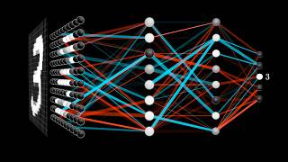


![Machine Learning with Python Full Course [2025] | Machine Learning - Beginner to Advanced | Edureka](https://img.youtube.com/vi/1fcfZ_Ne8ok/mqdefault.jpg)