hello everyone and welcome again to nettle the best platform around for distance learning in business finance economics and much much more please don't forget to subscribe to our channel and click that bell notification button below so that you never miss fresh videos and tutorials you might be interested in many thanks to our current patreon supporters for making this video possible and would also greatly appreciate if you consider supporting us as well so please check the link in description for more details my name is sava and today we're continuing to discuss various advancements generalizations and improvements
over the original garage framework and today we're investigating the e-gosh or exponential gauge model developed by nelson in 1991 and we can see that it makes quite a lot of changes with respect to the original gosh variance equation here in the original gosh we had our conditional variance vt squared being just a combination of unconditional variance omega the immediate disturbance epsilon t minus 1 squared and the persistence of variance v t minus 1 squared represented by alpha and beta parameters respectively and notably in the garage framework all three of the parameters were required to be
positive in egos many of these restrictions are relaxed and it is achieved by implementing not the usual vt squared as the dependent variable in the conditional variance equation but the natural logarithm of it over here it means that the natural logarithm of this variable can be either negative or positive that would lead to positive variance regardless so parameters omega alpha theta and beta can be potentially of any signs and that would be interpretable in terms of the volatility process furthermore it accounts for the asymmetric nature of volatility by implementing a structure of terms very similar
to tgosh that we have investigated in one of the previous videos so please check this out if you're interested in tigas so please check this out if you're interested in tigarch most of all however here we still got our alpha and theta parameters that have uh as their dependent variables the scaled a lag residual uh e t minus one divided by v t minus one so it's basically lacked disturbance scaled by lagged conditional uh standard deviation and the absolute value of such scaled lagged disturbance and again as in standard gauche you have got the volatility
persistence term beta but here it's also expressed in terms of the natural logarithm of lagged conditional variants this allows to accommodate for both the explosivity of variance behavior and the asymmetry of volatility clustering as well as relieves most of the restrictions on parameters in the original gauche framework and in terms of the maximum likelihood estimation it is still the same we can still express it in terms of the probability density function of the normal distribution with realized variance epsilon t squared and conditional variance vt squared as well as conditional velocity vt going into the equation
as arguments and we will maximize our log likelihood based on our five model parameters which are the mean the constant mu uh the log unconditional variance here it's interpreted as the natural logarithm of unconditional variance quite unsurprisingly given the mathematical expression of the conditional variance equation and our usual uh alpha beta and theta which is very similar to t gauss actually so let's start coding our e-gosh in excel and see how we can optimize the parameters so first of all let's start with the constant volatility assumption as usual and try to improve upon that to
do that let's just post our constant at first to be equal to simple average return over the whole sample our logarithm of unconditional variance would be just the natural logarithm of constant variance over here and we can just paste that like that and then we can input zeros as all three persistence terms alpha theta and beta and that would accommodate the constant volatility assumption the long run volatility in the egarch framework can be calculated first of all as the exponent simply because you've got a natural log over here of your log unconditional variance over 1
minus beta that would give us our long run variance and the long run volatility can be given as a square root of that and we can see that we have arrived at exactly the same uh value as we did when just calculating the constant uh volatility which is a welcome sign it means that even in the egash framework you can still improve upon your constant volatility assumption and see how persistence terms can improve the explanatory power of the volatility process without further ado we first need to calculate our residuals for every single observation so to
calculate the residual we need to subtract the constant mu from the realized value of return in every single day locking the new straight away then we can calculate our squared residuals and here we only need that for our log likelihood function as residuals go without squares in the conditional variance equation nevertheless we need them for this particular optimization to a task and then we need to input lagged residuals so no black squared residuals but just the lag residuals over here then we can start calculating our conditional variance and just as with usual garage models we
need to start with some value that is most often assumed to be equal to the long run variant so long run volatility squared and then we can start implementing uh our conditional variance equation with our natural logs so as we express the natural log of conditional variance we need to code our conditional variance as an exponent of this expression on the right hand side so first of all we're inputting the log unconditional variance omega rho locked here plus the arch term alpha that would be multiplied by the absolute value of lagged residual divided by lagged
conditional volatility so the square root of lagged conditional variance then we need to add our asymmetric term theta locking the row here as well and multiplying it by the value of the same scaled disturbance without the absolute value taken so that would account for asymmetry just as it does in the tigar framework so a lagged residual over that conditional volatility square root of conditional variance and then we need to add our agar term our conditional variance persistence term b9 and lock the row here as well and multiplied by the natural logarithm ln of lagged conditional
variance and then we can already enforce this formula and bottom wrap it all the way down and see that in case these three persistence parameters are zeros and our log unconditional variance is equal to the natural logarithm of constant variance we have got the constant variance assumption constant volatility assumption reinforced throughout the sample and graphically we can see it as just a straight orange line representing our egos configuration straight away and we can see that we have got our baseline garage estimations over here to compare our egarch results to the standard garage results so we'll
see if we can achieve a better fit graphically and in terms of log likelihood but to calculate our log likelihood we need to implement the probability density function with conditional and realized variance so let's just do that we need to input 1 over the square root of 2 pi and then we need our conditional volatility in the denominator so we'll just put conditional variance under the square root and that will achieve the desired objective and then we need to multiply it by this exponent term so times the exponent of minus squared residual which is realized
variance over two times the conditional variance vt squared over here and that would do the job so to get our log likelihood we can just calculate the natural log of this expression and to make the algorithm converge without crushing on calculational errors we can implement if error function over here and return a negative number a very high magnitude negative number so that the algorithm knows that errors are to be avoided so for example minus a thousand just as we did with a lot of various advanced garsh models and now we can watermark it all the
way down and calculate our total log likelihood as the sum of log likelihoods throughout the observations and we can see that this log likelihood is the same as we obtained from the constant volatility assumption previously which is a good sign um it is welcome now we need to calibrate our model parameters mu omega alpha beta and theta to arrive at the most at the highest value of log likelihood possible and then we'll see whether the goodness of fit whether the explanatory power of our ego model is greater than that of the simple garsh model and
we can even compare it to tigas why not so then let's go data solver and specify our optimization task we need to uh input log likelihood as our objective function we need to maximize that by changing variable cells with our five egarch model parameters so b5 to b9 mu omega alpha theta in beta and given the fact we have implemented uh this caveat that uh if there is an error return minus a thousand we can untick uh all of the boxes and again provided for the fact that egarsh relaxes a lot of the restrictions on
coefficients omega can be negative alpha and theta can be negative and so on and so forth and we can solve this task using geogen nonlinear using gradient descent so we can just click solve and wait until our model arrives at the optimal solution so that will take some time and our algorithm has just converged to the optimal parameter values that maximize our log likelihood we can see that our log likelihood is over 4400 which is substantially higher than the log likelihood of the standard garsh model and it's even higher than the log likelihood of the
tgarch model meaning that egosh does account for the dynamics of volatility to a greater extent than those simpler elaborations of the volatility process if we look at the coefficients and try and interpret them we can see that our long run volatility is again lower than our constant volatility assumption and comparing it to garsh and tigas we see that our egarch long run volatility is lower meaning that in the egos framework we would relax to lower values of long run volatility if there are no disturbances which is again a welcome sign meaning that we capture the
troughs of uh the volatility dynamics to a better extent we can see that our uh conditional variance is quite persistent with beta quite close to one and there is notable asymmetry in initial disturbance responses with some response to the absolute disturbance absolute scale black residual and there is a negative theta term over here which means that negative disturbances contribute to greater extent uh to the conditional variance persistence than positive disturbances and that's also in line with teargash assumptions and some stylized facts about how volatility clusters and behaves here omega the optimal value of omega parameter
is negative which shouldn't be surprising for you simply because uh omega is the logarithm of unconditional variance so that cannot be interpreted as some minimum value of variance the only way you can interpret it is by plugging in into the long run volatility calculation so let's see how well does the egash model proxy the historical dynamics of volatility over here on the graph and we can see that the orange line of egash does quite a better job than the standard gosh in grey with again relaxing to further extends uh in the volatility troughs and sometimes
a better proxy our volatility peaks that reinforces the notion that egosh can account for both the asymmetries in the volatility dynamics and the explosivity of the volatility dynamics by accommodating the natural logarithm function and that's all there is for the nelson exponential gosh or egarch model and its implementation in excel for volatility modelling please leave a like on this video if you found it helpful in the comments below i'll make you to see any further suggestions for videos in business economics or finance topics you would like me to record and please don't forget to subscribe
to our channel consider supporting us on patreon thank you very much and stay tuned