So, in this module, we are going to further discuss Work conjugacy. We will discuss Different stress tensors, and finally, we will look into some of the stress rate measures ok, and with this module, we will complete our discussion on stresses equilibrium equations, that is, the whole topic of kinetics ok. So, the contents of this module are as follows we will first look into the concept of work conjugacy ok followed by a detailed discussion on the First Piola-Kirchhoff stress tensor, and this, we will follow it up with a discussion on Second Piola-Kirchhoff stress tensors, ok.
And then, we will look into various ways in which the different stress tensors can be decomposed ok, and this will be finally followed by a detailed discussion on some of the objective stress measures ok and if the time permits, in this module, we will solve some examples in the end, ok. So, let us begin, ok. So, recall that from our previous lectures that the spatial virtual work equation was given by the following expression ok.
The internal virtual work was equal to the external virtual work ok. So, this is the internal virtual work, and this is the external virtual work ok. So, the total virtual work was the difference of the internal virtual work and the external virtual work.
So, the internal virtual work was defined as the integration of the internal energy over the current configuration of the body, ok. So, the internal energy is nothing but the double contraction of the Cauchy stress with the rate of deformation tensor, ok. The external virtual work can be thought of as having two contributions, as we discussed in the previous lectures, and this I am here just recapitulating what we already discussed so that we have a flow for today's lecture, ok.
So, the external virtual work is the sum of external virtual work because of the externally applied traction and the virtual work because of the body forces ok Now, the external traction virtual work is given by the summation over the current surface of the work done by the externally applied tractions on the physical surfaces of the body ok and the external body virtual work expression is nothing, but the work done by the body forces over the current volume of the body, ok. So, now let us now concentrate on the internal virtual work expression, which is given by the following expression, ok. So, this pair of second-order tensors, which is the Cauchy stress and the rate of deformation tensor d, they are said to be work conjugate with respect to the current volume B.
So, if you notice this expression of internal virtual work that was nothing, but integration over the current volume sigma d dV, ok So, this pair of second-order tensors, sigma, and d, is said to be work conjugate with respect to the current volume ok because the integration is being carried out over the current volume ok. So, what does work conjugate mean? Work conjugate means that the product of the two tensors ok.
In our case, the Cauchy stress tensor sigma and the rate of deformation tensor d give us the work per unit current volume ok. So, if you have two tensors and the double contraction of the two tensors gives you the work per unit current volume of a reference volume, it is called these pair of second-order tensors we will be called the work conjugate tensors, ok. From this internal virtual work expression, let us see how we can get some other measures of stress ok.
So, this equation 105 OKs is expressed in the reference configuration ok. So, now, this expression ok 105 ok see this is expressed in the current configuration. So, this is the current configuration, ok.
Now, if you express this expression in the reference configuration, then we can get alternative work conjugate pair of stresses and strain rates ok. So, now, if we just change the domain of integration from the current configuration to the reference configuration, we will get some other measures of work conjugate stresses and strain rates, ok. So, our objective is to see what are these different stress and strain rates, ok.
So, recall that the spatial volume element is related to the material volume element by following relation dV equal to Jacobean times dV 0, ok. So, now, if we substitute this expression in equation 105 7 or 8, then what we will get? We will get the internal virtual work ok as.
So, this was the expression, and if dV becomes JdV 0, then the domain of integration changes from the current configuration to the reference configuration, which is B 0 ok. So, we get integration over B 0 J sigma double contracted with the rate of deformation tensor times dV 0, ok. Now, we can define J sigma as another tensor called the Kirchhoff stress tensor ok.
So, this tau is defined as the Kirchhoff stress tensor, ok. Why we have done it? This is because if you look closely at this expression, ok, let see we had only stress contracted with a strain measure, ok.
So, here in the next expression, what we are getting there is a Jacobian which also comes. So, what we do? To make it consistent with this expression, we define what is called Kirchhoff stress tensor ok.
So, Kirchhoff stress tensor is given by J times sigma, ok. So, therefore, if you see Kirchhoff stress tensor is work conjugate with the rate of deformation tensor, but over the reference volume ok. So, Kirchhoff stress tensor is work conjugate to the rate of deformation tensor d with respect to the initial volume or the reference volume ok.
So, sigma or the Cauchy stress was work conjugate with the rate of deformation tensor with respect to the current volume. The Kirchhoff stress tensor is work conjugate with the rate of deformation tensor in the reference configuration ok. So, that is the difference.
Although body stress measures the Cauchy stress and the Kirchhoff stress, they are both work conjugate with the rate of deformation tensor, but one is work conjugate with respect to the current configuration while the other is work conjugate with respect to the reference configuration ok. So, that is what we need to remember, ok. Now, similarly, we can express the external virtual work corresponding to the body forces ok in terms of the reference configuration ok.
So, now, we know that the external virtual work because of the body forces is given by the following expression. And in this, if we substitute dV as Jd V 0, we get J b dot with virtual velocities integrated over the reference configuration, ok. So, we can define jB as b 0 ok.
To be consistent so that this equation is consistent with this expression ok. So, you have one vector dot with another vector, ok. So, that b 0 is Jb ok.
Now, the external virtual work also we can express in terms of reference configuration, ok. So, this is the external virtual work because of the surface forces and is given by integration of the work done by the tractions over the current surface, ok. Now, I can transform this to the integration of what we say as the reference tractions doing work over the reference configuration dA.
So, how did we get this? This we got by using what is called the formula that we derive. Remember from Nanson's formula da equals JF inverse transpose d capital A or nda was JF inverse transpose N dA, ok.
So, if you remember, when we were discussing kinematics, this was one of the examples that we did ok. So, this reference traction is nothing, but the actual traction times the ratio of the areas ok. So, this you can very well show ok now.
So, this, if you substitute here, if you substitute it here, you will be able to obtain this particular expression ok. So, this da can be obtained by the following relation, and this we derived earlier when doing kinematics, ok. So, we note that the work done per unit current volume is not equal to the work per unit initial volume ok that we will see ok.
However, from the continuity equation ok that we discussed in the previous lectures, the reference density is connected to the current density by this relation, ok. So, and the Kirchhoff stress is related to the Cauchy stress using the following relation, therefore, Kirchhoff stress. So, from here, J is rho 0 by rho, ok.
So, that is what we substitute here, and we get Kirchhoff stress in terms of the densities in the reference and the current configuration and in terms of the Cauchy stress, ok. So, the ratio of the Kirchhoff stress tensor ok and the current density is the same as the ratio of the Cauchy stress with respect to the current density, ok. So, now, if you double-take the double contraction with respect to the virtual variation of the rate of deformation tensor, you will get tau rho 0 double contracted with del d is sigma by rho double contracted with del d ok.
Now, if you use this in the internal virtual work expression, ok remember del w, ok. So, internal virtual work was B sigma contracted with del d dV. Now, if I divide by rho and I multiply by rho ok then rho dV is nothing, but the mass ok that is what we have here ok you have the mass ok.
Similarly, we had shown that the internal virtual work is tau del d into dV 0. So, if I take multiply and divide by rho 0. So, I have this and this relation over here nothing but the reference mass ok which is here, ok.
So, now you can see that both the integrals are the same; therefore, the integrants ok. So, they are the same; therefore, this shows that work per unit mass remains invariant ok because mass dM is the same as d capital M ok. So therefore, you will have work per unit mass which will remain invariant.
So, remember work per unit volume is not equal to the ok work per unit current volume is not equal to the work per unit initial volume ok. However, work per unit mass will always remain invariant ok because mass is neither created nor destroyed. So, this is how we have shown ok.
Now, this relationship over here is ok. So, 109, if we go back to this equation, if you see this expression over here, you see that these quantities, ok. So, this integration is in the spatial configuration while the integration is being carried out in the reference configuration ok.
So, you have to integrate the spatial quantity in the reference configuration, and this is a little inconsistent. So, what we will try to do now is we will try to remove this inconsistency, ok. So, what we do is to alleviate this inconsistency.
We start with the internal virtual work expression ok which is given by this ok, and then we note that DV is J dV 0. So, this I can substitute here, and then I can get integral over the reference configuration called double contraction of Cauchy stress with the rate of deformation tensor times J dV 0, ok. Now, another point to notice the double contraction of sigma with respect to the variation of the velocity gradient tensor ok can be written as sigma double contraction with the virtual variation of rate of deformation tensor plus the virtual variation of the spin tensor, ok.
Now, remember d is a symmetric tensor, and w is an anti-symmetric tensor. Also, we have shown from the law of conservation of angular momentum that in the absence of body couples, sigma is also symmetry which means sigma is equal to sigma transpose. So, we can show that the double contraction of a symmetric tensor with a symmetric tensor is not zero; however, the double contraction of a symmetric tensor sigma with the anti-symmetric tensor del w will be equal to 0.
So, del sigma del w will be equal to 0, ok. Therefore, this, when you open up this bracket, we get that the double contraction of Cauchy stress with the variation of rate of deformation tensor is the same as the double contraction of the Cauchy stress with the velocity variation of the velocity gradient tensor. So, this is the same as this and this is what we substitute here, and this is what we get, ok.
So, we now have this particular expression. Now, further, we note that the material time derivative of the rate of the deformation gradient tensor ok. F dot is said to be equal to lF.
This we had already derived. From here, I can say that the velocity gradient tensor l is equal to F dot F inverse ok. So therefore, del l will be the same as del F dot F inverse.
See variation will not be over F. Variation will be over F dot because its the F dot, which is changing with time. It's not F, which is changing with time, ok.
So, F you know ok at time t. Now when you apply a small displacement, F is not going to change, but F dot is going to change ok. Therefore, del l is del F dot F inverse, and this is what we have here, ok.
So, J sigma double contraction with del F dot F inverse, ok and this integrated over the reference configuration, ok. Now, we recall the property of double contraction of two tensors A and B, ok. What it says is that the double contraction of two tensors A and B, ok is nothing but the trace of A into B transpose, and it is also the same as the trace of A transpose B.
We are going to use this property in our integrand ok. Now, let us identify. So, if you see, we have a double contraction between two tensors, ok.
So, one second-order tensor is J sigma. The other second-order tensor is del F dot F inverse, ok. So, now, if I take A as J sigma and B as del F dot F inverse, therefore, I can write j sigma contracted with del F dot F inverse as the trace of AB transpose or trace of this is our A and this is B transpose ok.
So, I have written a trace of AB transpose. Now, the trace of AB transpose is the same as the trace of A transpose B, ok. So, now, I can write this as the trace of I can open up this transpose and I can write J sigma F inverse transpose del F dot transpose ok.
Now I can say A now is J sigma F inverse transpose and if I say B transpose is now del F dot transpose. Therefore, what we have here in the bracket is nothing, but the trace of AB transpose and the trace of AB transpose is same as see this is the trace of AB transpose is same as A contraction with B where A is J sigma F inverse transpose and B is nothing, but del F dot. So, using this here, I can write that the internal virtual work, when integrated over the reference volume, can be written as J sigma F inverse transpose double contracted with del F dot, ok.
Now, I can write this expression ok as P. I can denote this J sigma F inverse transpose as another tensor P, and then the internal virtual work becomes P double contracted with del F dot dV 0 ok where P is given by this particular expression, ok. So, in equation 119, this tensor P is work conjugate with the rate of deformation gradient tensor ok.
So, it is P is work conjugate with the rate of deformation gradient tensor with respect to the reference volume, ok. So, P is what we call the first Piola-Kirchhoff stress tensor. Some types of people also write it as first PK stress ok.
Sometimes people are also referred to as PK stress, or explicitly, we can call first Piola-Kirchhoff stress tensor, ok. Now, you can easily verify that P is an un-symmetric two-point tensor ok. So, first of all, if you take a transpose P transpose, it will be J sigma F inverse transpose, ok.
So, if you open this, J is the scalar. So, there is no transpose, F inverse transpose sigma transpose, ok. And then what you get is J F inverse sigma, ok.
Sigma transpose is the same as sigma, and this is not the same as the first Piola-Kirchhoff stress tensor. So, P transpose is not equal to P. Therefore, P is an un-symmetric two-point tensor ok.
So, it is a two-point tensor that, therefore, P in terms of its basis will be P i I E i tensor product EI, ok. So, equation number 120 can be written in indicial notation as follows, ok. P iI equal to J sigma ij F inverse capital I j ok, and you see P has one lowercase index and has an uppercase index.
So, it has two indexes. Therefore, it's a second-order tensor, and also it has one index, which is lower case, and one index, which is in the upper case. Therefore, it's a two-point tensor.
You can see from its basis also that one basis vector is from the reference configuration EI and the other basis vector, small e i, is in the deform configuration ok. So, it has it connects two different configurations. Therefore, it's a two-point tensor.
And its, but natural that a two-point tensor works conjugate with another two-point tensor which is nothing, but the rate of deformation gradient tensor because deformation gradient tensor itself is a two-point tensor, ok. Now, let us see now the virtual work expression can be expressed in terms of the first Piola-Kirchhoff stress tensor as the following expression. Remember initially we had del B sigma del d d V and now we have proved that this expression is the same as this expression over here.
So, therefore the virtual work expression takes the following form and then the governing equation that we had over here, ok. The divergence of sigma plus b equal to the residual force for all points inside the current configuration of the body will be changed ok to following expression ok. It will be changed to the following expression in the reference configuration, ok.
So, this is divergence, which means this is divergence with respect to the spatial coordinates, and this capital DIV means this is divergence with respect to the reference coordinates ok. So, the divergence of P plus b 0 is equal to r where it is X belongs to, ok. So, it is valid for reference configuration ok where divergences P is del 0 P double contracted with I, and del 0 P is nothing, but del P by del X ok.
So, now remember that the first Piola-Kirchhoff stress tensor was defined such that the internal virtual work expression in the reference as well as the deformed configuration; they both had similar analogous form ok which means there was stress in the deformed configuration and there is stress in the reference configuration there is a measure of strain in the deformed configuration, and there is a measure of strain ok here. So, we defined our first Piola-Kirchhoff such that we had an analogous form of internal virtual work expression ok in the reference or the deformed configuration ok. So, what it means is that the first Piola-Kirchhoff is just another mathematical representation of the Cauchy stress tensor, and P has been defined just for our convenience.
So, there is nothing physical about P, ok. The only physical stress tensor is the Cauchy stress tensor, but we have defined P for our own convenience ok and just purely a mathematical representation ok; that means, P is not any new physical quantity ok. Now, let us re-examine the physical meaning of the Cauchy stress tensor and the first Piola-Kirchhoff stress tensor ok.
So, what does Cauchy stress tensor actually mean ok physically, and what does the first Piola-Kirchhoff stress tensor actually mean? We will try to connect this to our undergraduate definitions of true stress and engineering stress. That is what our objective is, ok.
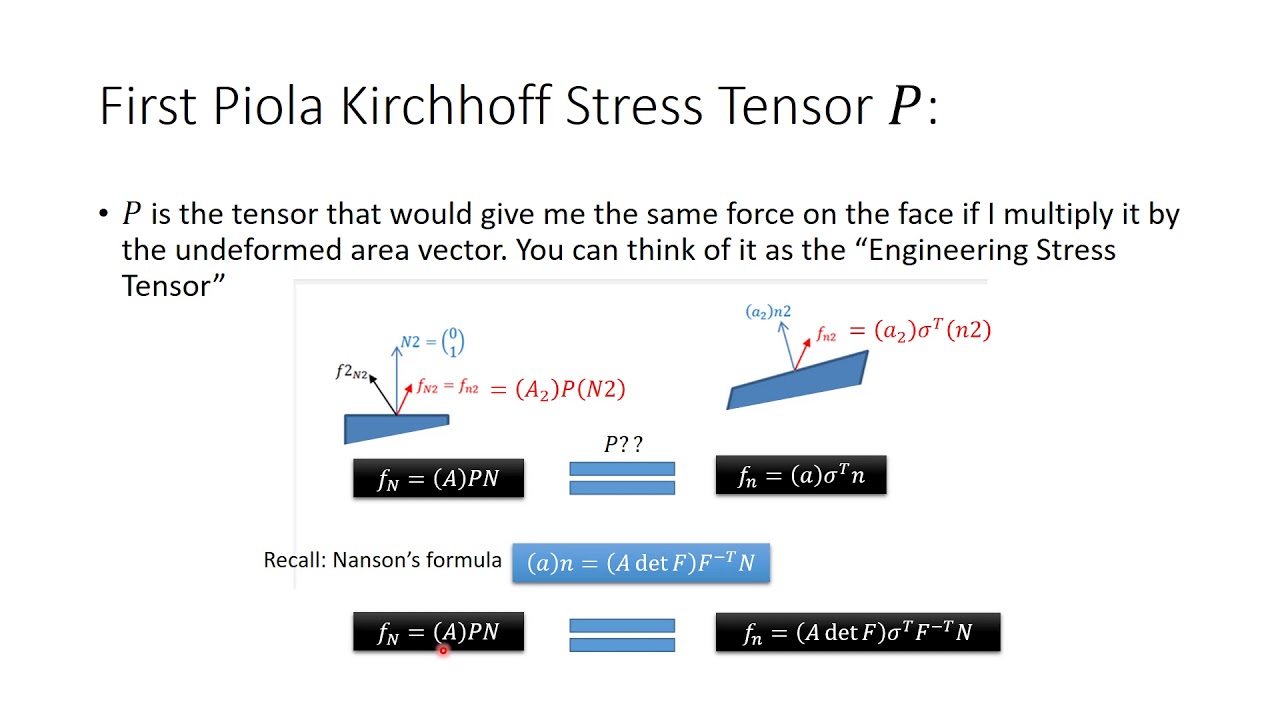
So, let us say you have a body in the reference configuration, and you have cut it open. So, you had a body like this, ok, and you had cut it open across a certain plane, and the normal to that plane is N capital N, and the traction vector is T, and the force along that traction vector direction is del P. So, del P del capital P is the force.
So, the area infinitesimal wall area ok reference area is da and when the deformation happens the body occupies this configuration ok B ok. So, this is B 0. So, the area is da, the normal to the area is n, the traction vector is t ok, and the force vector along t is dp, ok.
So, now we consider an element of force dp, in the spatial configuration acting on the current area d a and the current area vector da is nothing, but the normal to the area times the magnitude of the area ok. So, n da ok. So, now, the force dp is nothing but the stress factor times the area on which it acts.
So, t times da. Now, from the Cauchy stress principle, we know that t is equal to sigma n ok because we know t is equal to sigma n. So, because of the Cauchy stress principle, I can relate to the traction vector at a point ok on a plane whose normal is n using Cauchy stress principle ok.
So, sigma n d a. Now nda is nothing but the area vector. So, the force is Cauchy stress times the current area is ok what it means is loosely we can say ok.
So, if you see here, dp is sigma d a, ok. So, loosely we can say that the Cauchy stress is equivalent to the current force; this is the current force per unit current area. So, d is the current area.
So, if you can loosely say that sigma is like dp by d a, ok loosely because they are both vectors, I cannot take this ah ratio. But I can loosely say that Cauchy stress is the ratio of current force to the current area, and this is synonymous with our definition of true stress. Ok, that is how in our undergraduate, we define true stress.
It is the current force divided by the current area. Therefore, Cauchy stress is also called true stress. Cauchy stress would be true stress, ok.
Now, I can use Nanson's formula ok in equation 127. I can write the spatial area element da in terms of the material area element d capital A by this Nanson's formula. If I substitute this expression in expression number 127, then what I get?
I get dp is tda equal to J sigma F inverse transpose d A. Now, from a previous slide, we know that J sigma F inverse transpose is nothing, but the first Piola-Kirchhoff stress tensor P ok . So, the current force is equal to the first Piola-Kirchhoff stress tensor P times the reference area d A, ok.
So, loosely I can say that P indeed is a two-point tensor. So, now the two-point tensor, which might not be clear when I said it in the previous slide to you, will now become clear. You can clearly see that P maps the area vector in the reference configuration to the force vector in the deformed configuration.
So, that is a two-point tensor rate. It maps one vector in one configuration to another vector in another configuration. So, P is the first Piola-Kirchhoff stress tensor.
Is mapping the reference area element ok to the force in the current configuration ok. So, that shows the two-point nature of the first Piola-Kirchhoff stress tensor, and this relates the area vector in the initial configuration to the force vector in the current configuration ok. Therefore, loosely I can say P is nothing but current force divided by reference area or the undeformed area and which is our usual definition of the engineering stress or the nominal stress.
So, P can be interpreted as equivalent to the engineering stress or the nominal stress that is current force per unit undeformed area ok. Now, we know that the area vector in the reference configuration is given by the normal to the area dA times the magnitude of area d A-ok. Now I can write ok in expression 128, I can substitute da as N dA, and then the current force is equal to PN times d capital A-ok.
So, if I divide both sides by dA then I get dp by dA is equal to PN, and I have defined dp by dA as the nominal traction T ok. I can define dp by dA as a nominal traction T, then I can get dp by dA is equal to T equal to PN, and this is nothing but the material form of the Cauchy stress principle. So, this t equal to sigma n was the spatial form of the Cauchy stress principle, and capital T equal to PN is nothing, but the material form of the Cauchy stress principle is ok.
Now, we can get the material form of the balance of angular momentum ok. So, we know that the first Piola-Kirchhoff stress tensor is not symmetric, but from our discussion on the balance of angular momentum, we had shown that the balance of angular momentum in the spatial configuration resultant in the statement that Cauchy stress tensor is symmetry. However, now let us say what happens when we take the balance of angular momentum in the material form ok.
So, we start by looking into the implication of the balance of linear momentum in the current configuration, and the following was the expression if you remember that we derived. So, epsilon ij k sigma kj integrated over the current volume should be equal to 0, or this integrand can be written as the alternator symbol contracted with Cauchy stress tensor ok. So, if I just substitute, I have this particular expression, ok.
Now I know that P is J sigma F inverse transpose ok. So, from here, sigma F inverse transpose will be 1 by J P ok . So, if I multiply both sides by F transpose, I will get sigma is 1 by J P F transpose.
Now, if I substitute for sigma in this expression, ok over here, I will get what is written over here ok, and now I can substitute dV as JdV 0. So, this becomes integral over the reference configuration epsilon contracted with PF transpose ok dV 0 ok. So, therefore, in a similar way as we did for the Cauchy stress tensor, I can show ok, and this I leave it for you as an exercise to show that PF transpose will be equal to PF transpose, which means that PF transpose will be symmetric ok.
So, PF transpose is FP transpose ok . So, this is the implication of the balance of angular momentum in the material configuration. Remember, in the spatial configuration, the implication of the balance of linear momentum was that the Cauchy stress tensor came out to be symmetry.
However, our first Piola-Kirchhoff stress tensor is not symmetric, but in the material form of the balance of angular momentum, the derivation that we did just now shows that PF transpose is the same as FP transpose; therefore, PF transpose is symmetry although P itself is not symmetry, ok.