Lecture 15: Coding the self attention mechanism with key, query and value matrices

[Music] hello everyone welcome to this lecture in the build large language models from scratch Series today I'm very excited for this particular lecture because today we are going to look at implementing a self attention mechanism with trainable weights we are going to look at Key query and value and we'll also see why this self attention mechanism is also called as scaled do Product attention so we are now moving very closer and closer to the actual attention mechanism which is implemented in LMS such as GPT today's lecture will be a great combination of mathematics uh Theory

intuition and also coding I really enjoyed learning so much about this lecture and preparing the lecture material and I've condensed all the information in today's video so let's get started before we get started I want to quickly touch upon what we covered in the previous lecture in the previous lecture we implemented a self attention mechanism without trainable weights so this is the uh sentence which we looked at the sentence which we looked at was your journey starts with one step and we saw how to convert the embedding Vector the vector embedding for every single token

into a context Vector for every single token and uh let me take you through the Steps we implemented to do that and I'll go to the figure which really illustrates everything yeah so what we did essentially in the last lecture was that we broke down the initial sentence into the embedding vectors which were three-dimensional input embedding vectors and then we looked at queries so we took the example of let's say Journey which is the second query your journey begins with one step and then for each such query we found the attention scores With respect to

the input embedding Vector so for the first word there is a attention score between the first word and the query for the second word there is a attention score similarly for the last word there is a attention score this attention score actually quantifies how much importance should be given to each word when we look at the query which is Journey and then based on these attention scores we found the attention Weights the difference between the attention weights is that attention weights sum up to one so attention scores and attention weights intuitively mean the same thing

the encode information about how much the query vector and the input embedding Vector are related to each other and attention weights are normalized which means they sum up to one the way we computed the attention scores is by implementing a DOT product Operation so what we did is we implemented a DOT product between the query vector and the input Vector so let let me show this to you um in figure so that you have some reference to compare yeah so what we did essentially was we had this uh Journey which is the query Vector to

find the attention score we found the dot product of this Vector with all the other vectors and that give the attention scores then we normalize the attention scores to give the to get The attention weights and then finally we use the attention weights to find the context Vector so here is the context Vector for Journey and similarly we found context Vector for all the other vectors for all the other input tokens so uh the steps which we implemented in the last class can be summed up in three uh categories first we computed the attention scores

for that we computed the dot product between the inputs and the query then we computed attention Weights which were normalized attention scores and then we computed context vectors so context vectors are essentially the weighted sum of the attention weights and the input vectors so here's a figure which explains how we found the context Vector so we found the attention weights for the given query and then let's say the first attention weight was multiplied by the first input Vector the second attention weight was multiplied by the second input Vector Similarly the last attention weight was multiplied

by the last input vector and we added all of these vectors to give us the context Vector for that given query in a similar manner we found the context Vector for all the other queries in the given sentence so this is what we implemented in the last lecture and we did not have any trainable weights we did not train anything in the last lecture everything was fixed the attention scores was Calculated using the dot product um the attention weights was just normalization and the context Vector was just summation of the uh attention weights multiplied by

the corresponding input Vector today we are going to look at a more real life situation which is actually implemented and we are going to consider trainable weights if you have not seen the previous lecture I highly recommend you to go through the previous lecture you'll appreciate the current Lecture much much more okay so in this section we are going to learn about the self attention mechanism which is used in the original Transformer architecture the GPT models and most other popular large language models the self attention mechanism is also called as scaled do product attention and

in this lecture we are going to see why this name comes into the picture and where this name is derived from I'm following this particular Sequence in the attention Series in the last lecture we covered simplified self attention in today's lecture we are going to cover self attention with trainable weights in the next lecture we'll look at causal attention and in the final lecture we look at multi-head attention as I explained in the previous lecture also it's impossible to cover attention in one lecture that's why I have designed these extensive lectures to teach you the

concept in a very Proper manner it might get a bit complex at times but if you understand the concept you will Master Transformers because this is the heart this is the engine of Transformers and I'll show everything from scratch right up to the last dot product I'll multiply all matrices directly in front of you so that you understand matrix multiplication it's very important to do things on a whiteboard because then the Understanding is improved much more okay so what we want to do in today's lecture is that we want to compute the context Vector for

every given input token so the objective of today's lecture is the same as the objective was in the last lecture remember what we did previously in the previous lecture we found we took this sentence your journey starts with one step we we had the input embedding Vector for each of these tokens and then We found a context Vector for each of these tokens so this graph here shows the input embedding Vector for every token and the red the journey context it shows the context Vector for Journey similarly we found the context Vector for all the

other input vectors to refresh your understanding the context Vector can be thought of as an enriched input embedding Vector so if you look at the word journe here the embedding Vector for Journey uh the embedding Vector for Journey Only in encapsulates or encodes the semantic meaning but it really contains no information about how that word Journey relates to the other words right the context Vector for Journey on the other hand has more information it not only contains the meaning of Journey but it also contains how Journey relates to step your with and one that's why

the context Vector is thought of as an enriched embedding vector Awesome so today what we are going to do is we are going to introduce weight matrices which are eventually optimized when the large language model is trained now these trainable weight matrices are very crucial because the model then learns to produce good context vectors in the last lecture we just uh looked at context vectors by essentially taking the dot product to get the attention weights that's it right we did not train anything but We'll see how these train weight matrices are constructed and once these

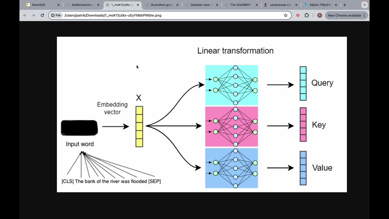
weight matrices are trained the model can learn to produce good context Vector for every token so at the heart of this trainable weight matrices are three terminologies query key and value let me repeat that again we are going to implement the self attention mechanism step by step by introducing three trainable weight matrices the First is called the weight Matrix for query the second is called weight Matrix for key and the third is called the weight Matrix for Value so these three terminologies will show up again and again and again query key and value and let

me show you a diagram which illustrates what these terminologies actually mean so uh here I have mentioned here step number one step number one which we are going to learn in today's lecture is How to convert in input embeddings which are the input vectors into key query and value vectors remember the goal here is the same as the last lecture we want to get from the input embeddings to context embeddings for every token but there are number of steps to be done and the first step here is to convert the input embeddings into key query

and value vectors let's see what we mean by that and how to get these key query and value vectors okay so here are my Inputs your journey start with one step right these are my uh six inputs and I've represented these six inputs as threedimensional vectors which you can also see in the graph below so if you look at the input Matrix the first row of this Matrix represents the three dimensional Vector for y the word Y the second row of this Matrix represents the three-dimensional Vector for Journey which can also be plotted here similarly

the last row represents the Three-dimensional Vector for the input word or the input token step right this is how the input embeddings are that's given to us now the next step to construct the query key and value Matrix is to look at three trainable weight Matrix the first trainable weight Matrix is called as the query weight Matrix the second trainable weight Matrix is called as the key weight Matrix and the third trainable weight Matrix is the value weight Matrix so what we going to do is That let's look at these weight matrices uh and let's

also focus on the dimensions here so the input has Dimensions 6x3 because there are six rows one row for each input token and why three because the dimension Vector Dimension size is three now let's look at uh uh the query key and value trainable weight matrices so this W key W uh WQ W K and W V these three matrices which I've written over here I've initialized them with some random values But these are the ones which are actually trained we do not know these parameters so we initialize them randomly and then train them so

to get context vectors later which we'll see in today's lecture these are the ones which are optimized now what these uh matrices do is actually they project the inputs into a different dimension space let me tell you what I mean by that so first let's focus on the qu query Matrix so if you Look at the query Matrix and if you see the dimensions it's 3x2 uh so it has three rows and two columns so if you multiply the inputs if you multiply the input Matrix with the query weight Matrix what you will get is

the resultant Matrix which is called as the queries so this is the queries Matrix and it's a 6x2 matrix so what has been done essentially is that each row here still corresponds to the individual words so the first row corresponds to Your the second row corresponds to Journey the third row corresponds to begins with one and step but you can see here that the dimension has been changed usually when we train GPT the dimension is preserved but here I'm just illustrating that the dimensions can be changed when you multiply with the weight query Matrix so

the simplest way to think of the query Matrix and all the other weight matrices is the transformation from let's say a Threedimensional space into in this case a two- dimensional space uh so when we multiply the input Matrix with the query weight Matrix we get the queries Matrix which is a 6x2 matrix okay so now you can think of each row as corresponding to the corresponding input token your journey begins with one step the second weight Matrix is the key weight Matrix and that's all also 3x2 Matrix and very similar to what we did For

the queries we'll multiply the inputs with the keys weight Matrix and then finally we'll have the keys Matrix which is again a 6x2 we'll see what these different uh matrices mean what's the meaning of query key and values but for now let's just look at the mathematical details of the implementation right and similarly to get the values to get the values Matrix we have to multiply the inputs with the weight Matrix for values and The weight Matrix for values is also 3x2 Matrix and when we multiply the inputs with values we again get a 6x2

so the way to interpret the uh query key and the value is that every row of the query key and value essentially represents one token and a representation for that token so henceforth after we get the queries key and values we are not going to look at the inut embeddings again the input embeddings have been transformed into Three ve into three matrices the query the query Matrix the key Matrix and the value Matrix and remember this transformation is not fixed the key the key to these Transformations are these three weight matrices WQ w k and

WV the parameters of these weight matrices are to be optimized later that's why these are called as the trainable weight matrices for now just think that what we have done in this first step is we have taken the input Matrix and we have Converted the input Matrix into three other Matrix matrices queries keys and values and the way we have done that conversion is by multiplication of the input embedding with the trainable query Matrix with the trainable key Matrix and the trainable value Matrix and so we have these three queries keys and values Matrix which

is constructed so you might be thinking why do we have these three and how do we get the attention scores how do we get the context vectors don't Worry we'll come to all of that but first let's go to code and let's try to implement uh all of these okay so I'm going to take you through code right now so the first thing is to construct the inputs so we'll have as I mentioned the inputs is essentially a matrix which has six rows uh it has six rows and it has three columns so that's what

I'm going to Define here the inputs is a tensor with six rows and three columns so each row Corresponds to a particular word let's say journey is a three-dimensional Vector so I'm going to run this right now and you'll see that this block has been run and what we are going to do is that the next thing what we are going to do is initialize the query key and the value query key and the value Matrix query key and the value weight Matrix right and for that we need to define the dimensions right so uh

here the dimensions are 3x2 the three has to be Equal to the vector dimension of the input so that has to match because we are doing a matrix multiplication here so for all of these three weight query key and value weight Matrix the first value of the dimension three has to match the vector Dimension but the second dimension can be anything so uh if you when you initialize the query key and the value we are initializing random values and the shape of the Matrix is D in comma D Out remember D in is just the

shape of the input so we are just looking at one particular Vector of the input that's the vector Dimension three so that's also the first uh argument of the shape of the key query and value Matrix this exactly what we saw here this first argument has to be same as the uh Vector Dimension which is three and the out Dimension we are choosing to be two in this case so note That in GPT like models the input and out output dimensions are usually the same but for illustration purposes we are choosing the input Dimension is

three and the output Dimension is two over here so these are the query key and the value weight matrices and each element in these weight matrices has been initialized in a random manner so you can actually see tor. nn. parameter and you can see the documentation for this uh yeah so what so you can see what It does it's uh so it's a kind of tensor that is to to be considered a module parameter and inside this you can pass some things so what we are doing is that we are passing the parameters to be

random values with the shape of D in comma D out which means that the Matrix shape for query key and value will be 3 comma 2 so you can print out the trainable weight matrices so this is the trainable weight Matrix for query it's a three three row by two column tensor This is the trainable weight Matrix for key it's a three row and two column tensor and this is the trainable weight Matrix for Value this again is a three row and two column tensor awesome uh some minor things is that we are setting this

requires grad right now to false but remember that uh later we are going to train the values in these matrices through back propagation so at that time we'll need to compute Gradients and at that time we'll set the requires grad to be equal to True great so now we have computed the key query and value um key Quant value weight trainable weight Matrix right now we have to do the multiplication of the inputs with these Matrix to get the queries key and values uh final Matrix so to do that first what we can do is

we can look at an individual element so let's say we look at this second element which is Journey and let's say we want To First convert this second element journey into its corresponding query uh let me show you how we can do that but first let me rub um some of the things here so that I can easily show you how we get the key query and value Matrix for Journey okay so what we are doing here is that we are focusing our attention um also let me change the color yeah so we are focusing

our our attention on this Second um input Vector which is Journey and then we want to get the query key and value Vector for Journey So currently the input Vector is a three-dimensional Vector now we need to get the two-dimensional Vector so the way to get that is look at these queries keys and values so the second row here will be the corresponding query Vector for Journey the second row here will be the corresponding key Vector for journey and The second row here will be the corresponding value Vector for journey so the way you get

the this second element is just you take the uh you take the journey and uh then you are going to uh dot product it with this uh weight Matrix q and similarly for key and similarly for Value so this is what we are going to see in code right now um instead of directly showing you The matrix multiplication first I wanted to show it to you for each individual element so remember this if you look at each individual element this is one row and three columns so we can multiply it with the query three row

two column and that will give us a one row two column which is the query Vector for Journey similarly for keys and values this is what I'm going to show you in code right now so uh let's look at the second Element X2 and X2 has been defined earlier as inputs accessed and the index is one so since python has a zero indexing system inputs one will essentially be the input for Journey so that is defined by xor2 so we are going to uh find the query corresponding to this xor2 by multiplying it with the

weight Matrix for query we are going to find the key for the journey vector by multiplying it with the key Matrix and we are going to Find the value for the journey vector by multiplying it with the value weight Matrix and here you can see we get 4306 and 1.45 51 which is the query Vector for uh so I'm just printing the query here so this is the query Vector for Journey and let's see whether it matches so the query Vector for Journey was indeed 43 and 1.45 here if you can see uh what I'm

showing in the color right now and that exactly matches what we have in code awesome so we are Currently moving in the right direction as we can see based on the output the result is a two dimensional t two dimensional vector now what we can do is that we can actually obtain the keys and values uh and queries for all the different inputs this is exactly what we had written over here once we get the trainable weight Matrix we can just multiply the inputs with these weight Matrix and get the get the queries Matrix get

the keys Matrix uh get the keys Matrix and get the values Matrix so this is what I'm going to show to you in code right now okay so to get the keys Matrix we just multiply the inputs with the weight Matrix for keys to get the values Matrix we just multiply the inputs with the weight Matrix for values and to get the queries Matrix we just multiply the inputs with the weight Matrix for query and uh let me just run this right now so If you run this you can just print out the shape of

the keys values and queries and as expected it's 6 by two so we have six rows and two columns uh why six because there are six input tokens your journey begins with one step and for each input token we have a twood dimensional key Vector two dimensional value vector and two dimensional query Vector so as we can tell from the outputs we have successfully projected the six input tokens from a 3D input Embedding space from a 2d embedding space for the keys values and queries okay so if you have understood up till now you have

essentially understood the first part of today's lecture and and the first part was how to convert input embeddings how to convert input embeddings into key query and value vectors awesome now we are ready to move to step number two and uh before that let me just show you a schematic of what we have done until now So what we have done is that we have the inputs right and we have converted the inputs into their embedding the threedimensional embedding vectors then what we did was we had a key query and value and we multip IED

every input with the key query and the value so here I'm showing keys and values so you can multiply every input with the keys queries and value to get the uh key query and value Matrix for every single input Embedding that's what we have done until now essentially every input embedding Vector has been multiplied by with the key query and value trainable weight Matrix to get the final key query and value matrices for all the inputs so for the rest of the lecture imagine that we don't have the input embeddings at all we will only

deal with the key query and value matrices so now let's move to the next step in the next step uh we have to compute the attention Scores what is meant by attention scores we have to essentially compute that if you are given a query U let's say if you are given a particular query uh how does the other Keys attend to the that query let me explain this to you so let's say uh we have the query for the second word which is Journey and this is the query which is a two-dimensional Vector now we

have to find out how does this query attend to the keys for the different input words so you can think Of the keys right now as just individual tokens like what we did in the previous class remember in the previous class the query was just the just that particular token we did not have a separate Vector for query we just the journey itself was the query the journey token itself was the query so if ever you get confused in terms of intuition just think of the query as being the token itself although it's a bit

different so what we are essentially doing is finding how that Particular query so now we are looking at query number two which is related to journey and we want to see how the other words attend to Journey which means that when I'm predicting the next word how much in importance should I give to your how much importance should I give to Journey how much importance should I give to with one and step so my query is Journey and I'm going to look at how much importance I need to give to the other words so that's

why we need to Find the attention scores between the query and the key remember this intuition is very very important right now what we are essentially doing is that we are finding the attention score between the query and the key in the previous leure we just found the attention score between the input embedding vector and the other embedding vectors by taking a DOT product but now remember we don't have the input embeding space at all we are In an abstract space we are in the query key and value space so we are going to find

how the query number two attends to the different key vectors and we are going to find it in the exact same manner as we did in the last class remember the mathematical operation which helps us to find whether two vectors are aligned or not that is the dot product operation so let's say if this is my query vector and if uh let me show the key Vector in some Other color so let's say this is my query vector and let's say this is my key Vector these two vectors are very much aligned with each other

right so the dot product will be maximum so it says that when I look at the query I should probably pay more attention to this key Vector whereas let's look at another key key Vector now which is like this so let's say there is another key Vector which is like this so now if you look at The query and this second key Vector they have a 90° angle with each other they are not at all aligned which means that when you look at that query you should not pay attention to this green key over here

and that is encapsulated by the dot product if you find the dot product between the yellow vector and the green Vector they have a 90° angles the dot product will be zero that's what we are going to do now we are going to find the the attention scores between The particular query and all the other Keys remember every every query will have an attention score with all the other keys so for example if you look at query number two for Journey it will have an attention score with key number one it will have an attention

score with the key number two and similarly it will have an attention score for the final key uh which is Step so this is what we are going to do next and let me show this to you in a Picture tutorial representation right now okay so the way we are going to do this is by initially only focusing on the queries and keys okay so let's say we look at so this is our queries Matrix which is a 6x2 and I'm going to now focus on the second row of this because I'm going to look

at Journey I'm going to look at the word Journey so the query for the word journey is the second row right now what I actually want to do is I want to find the uh dot product Between this query and all the other key so I want to find the dot product between this query and the first row with the second row with the third row with the fourth row with the fifth row and with the sixth row so to essentially find the attention score for the second query all we need to do is we

need to take the that particular row and we need to find the dot product with all the other rows of the keys so we'll have six attention Scores and that those attention scores contain the information that when you look at the query for Journey how much importance should be given to other words like your journey begins with one step so this is what we are going to implement in code right now so I'm going to look at the keys of one um so I'm going to look at this keys so Keys 2 is keys of

one which means the key for Journey uh which I have highlighted over Here so this this is actually my key Keys underscore 2 so the keys uncr 2 in the code is the keys for Journey uh and then what I'm going to do is I'm going to uh take the dot product between actually before that let me right yeah so let me correct that a bit so this actually is queries so this is actually queries unroll 2 so Query unroll 2 is is this query so let me reframe that again uh so here what I

have is query query uncore 2 and to find the attention score for this query I'm going to take a DOT product between the second query and the keys Matrix so this is exactly what has been done in the in the code here so to find the attention score between the query 2 which is the query for Journey we are going to take a DOT product Between the query and the keys transpose why are we taking a transpose here because look at the dimensions always look at the dimensions uh the dimensions for query is that it's

one row and it's uh it's one row and it's two columns so we cannot directly multiply it with the keys because the keys has six rows and two columns whereas keys transpose we have two rows and six columns and that can be multiplied so then Keys transpose will be 2x 6 so let me write that Dimension down so Keys transpose will be 2x 6 and if you multiply 1X two Matrix with 2x 6 you'll get 1X 6 so you'll get six attention scores for all the different uh for the six input tokens your journey begins

with one step so that sounds correct so this is what we are going to do over here so the attention scores two which is the attention score for Journey is just a matrix product between the query for Journey multiplied with the keys Transpose so you get the six attention scores here so as you can see the first attention score is the encodes information about how much Journey attends to your the second attention score encodes information about how much Journey attends to Journey the third attention score encodes information about how much Journey attends with width similarly

the last attention score encodes information about how Journey attends with step so the second score is The highest because of course journey and journey will be intuitively more aligned to each other but remember these scores don't mean anything right now because we have not trained any of the weight matrices these scores will only mean something when you train the weight matrices so ideally if you have a long paragraph and and if journey and step are more related to each other in that paragraph after the matrices are trained This last value which is the attention score

between journey and step has to be the highest so up till now what I showed you is how to find the attention score the six values of the attention score for one query but now what if you want to find the attention score for all the other queries for the first query second third fourth fifth sixth the simplest way to do that is just for the second query you just multiplied it with the Keys transpose right and similarly you'll do for all queries so why don't you just do a matrix multiplication so you multiply the

queries Matrix with keys transpose and I've shown this over here for your reference so this is the query's Matrix which is 6x2 and the keys transpose is 2x6 so of course 6x2 can be multiplied with the 2x6 Matrix and ultimately you'll get a matrix like this which is a 6x6 Matrix and that is our attention Score Matrix now what does this attention score Matrix symbolize so the first row is contains the attention scores between the first query and all all the other Keys the second row contains the attention scores between the second query and all

the other Keys similarly the last row contains the attention score between the last query and all the other Keys that's the simple meaning of the attention scores and I'm again going to Do this in code right now to get the attention scores I just take the matrix multiplication of queries with keys transpose and then you get the 6x6 uh attention scores Matrix that's it so we have calculated the attention score between every query with respect to all the other Keys awesome uh this is the second step and we have still not yet got to the

context Vector so the first step was to convert the input embedding vectors to the key Query and value the Second Step was to use the key and the query to get to the attention scores now the problem with these attention scores is that they are not interpretable right ideally I want to be able to let's say if I look at this second uh this second row which are the attention scores for the query journey I want to be able to make the statements like okay pay 10% attention to your pay 20% attention to Journey pay

30% attention to step pay 40% attention To width but I'm not able to make these interpretable statements because if you look at all these attention scores they do not sum up to one these look like random values that they are not summing up to one so we have to do the next step of normalization so normalization serves two purposes first it will help make things interpretable so I can make statements like okay when the query is Journey the you pay 20% attention to the First token 30% attention to the final token Etc and the second

advantage of normalization is that it helps when we do back propagation generally in many machine learning Frameworks it's better to normalize things so that the scale stay consistent between zero and one so the third step what we are going to do is that we are going to compute uh the is terminology which is called as attention weights so up till now we have calculated attention scores that's fine Now we are going to just normalize the attention weights uh so that the attention scores in each row sum up to one so there is a difference between

attention scores and weights the meaning is the same but attention weights sum up to one they are normalized in the previous lecture what we did for normalization is that we looked at each row and we simply took the soft Max right uh and the soft Max function actually ensures that all the Elements sum up to one I'm not going to cover the soft Max implementation in today's lecture because we have already seen it in the last lecture in a lot of detail but remember that softmax just make sure that all of the these quantities sum

up to one and they lie between zero and one and they are positive but actually in today's lecture before we Implement soft Max there is one more very important step which is actually done and I'll come to why this Step is done but remember that before implementing soft Max what is done is that all of these values are taken and they are scaled by something which is called as square root of the keys Dimension So currently the dimension of the keys is a it's two two Dimension right because remember the keys queries and the values

Matrix we uh we took the three-dimensional input embedding and we transformed it into two dimensional so the dimension of the keys In this case is two uh so we are going to to scale everything by square root of two why two because if you look at the um let's look at the key Matrix again yeah this is my key Matrix right now and if you look at every uh if you look at every token here it has two Dimensions right so that's why we are going to uh we are going to scale by square root

of two and you might be thinking okay this looks like magic who thought about the square root why do we do the scaling There is a very nice reason for that and I'm going to come to it for now just remember that after getting the attention score we are going to scale it by square root of D and that's why it's also called as scaled dot product attention remember we saw at the start the scaled we are going to scale by square root of D that that is one of the reasons why it's called scaled

dot product attention so we are going to scale it And then we are going to apply soft Max so when we scale by square root of two it leads to this Matrix over here and then we have apply soft Max so you'll see that when soft Max activation is applied and if you look at each row right now you'll see that they sum up to one so if I look at the second row right now uh it corresponds to again um Journey so I can now confidently make statements like when the query is Journey pay

15% attention to your pay 22% attention to Journey itself pay 22% attention to with to begins pay 30 15% attention to width pay only 9% attention to one and pay around 18% attention to step remember these weights are not optimized but when they are optimized we can make interpretable statements like these all of the rows will sum up to one you can check these and this is called as the attention weight Matrix this is one of the most important step uh in getting to the context Vector please Remember this step and uh we did two

things here we scaled by the square root of the dimension and then we implement soft Max now let's go go to code and let's implement this in the process we'll also understand why we do the scaling by square root of D okay yeah so we compute the attention weights by scaling the attention scores and using the soft Max function the difference to earlier when I say earlier It's the previous lectures is now we scale the attention scores by dividing them by the square root of the embedding dimension of the keys and that embedding Dimensions is

two so we are dividing by square root of two so let's do the same thing here so we have this attention scores 2 so it's a 6x6 Matrix which we have printed out here actually currently I'm just employing this on the attention scores for the second query okay no problem so Attention scores 2 is the attention scores for the query 2 which is Journey so it's actually one row and six columns so what I'm going to do is that I'm going to take this attention scores for Journey I'm going to first divide it by the

square root of the keys Dimension and then uh what I'm going to do is that I'm going to apply soft Max the reason we do dim equal to minus one is that because we have to sum over all the columns and all the if so that's why When you look at one row you'll see that it sums up to one so two things are important this D of K is the dimension it's the keys do shape minus one because we are looking at the column remember keys do shape is 3x 2 so when you do

keys do shape and index it by minus one the result will be two so we are going to uh divide by square root of two uh and in Python remember here we are exponen by 05 so into into .5 means rais to.5 that is the same as dividing by the Square root of two so every element will be first divided by the square root of two in the attention score and then we implement the soft Max so if you look at the attention weights for Journey you'll see that these are the attention weights let's actually

check whether these are correct to what we saw yeah so let's look at the second row here the second row is 0.15 2264 etc for Journey and here you will see that the second the Output is exactly the same that's a good sanity check and you'll see that all of this sum up to one so this is how we calculate the attention weights for one uh query and similarly we calculate the attention weights for all the queries so if I just replace this with attention scores which is the 6x6 we'll get the attention weight Matrix

which is a 6x6 Matrix okay now let's come to the question which all of you might be thinking and I don't think this is Covered enough in other lectures and other videos but it's a very fascinating thing I took some time to understand this and I've come up with two reasons why we actually divide by the square root of Dimension the first reason is stabil in learning and let me illustrate this with an example so let's say if you have this tensor of values which is 0.1 min-2 3 -2 and .5 okay if you take

the soft Max of this uh versus now let's say if you Multiply this with eight and then you take a soft Max so you'll see that the soft Max of the first is kind of it's good right it's diffused these values are diffused between 0o and one but if if you look at the soft Max of the second tensor you'll see that the values are disproportionately high which means that if there are some values in the original tensor if some values are very high and when you take the soft Max you'll get such kind of

peaks in the Softmax output I've actually explained this better here so the softmax function is sensitive to the magnitude of its inputs when the inputs are large the difference between the exponential value of each input becomes much more pronounced this causes the softmax out output to become pey where the highest value receives almost all the probability mass and we can check it here so when we multiply with uh8 you'll see that this has the highest value Which is four and when we take the soft Max you'll see that the value is 08 here which is

much higher than all the other values in fact it's around 10 to 15 times higher that's what is meant by softmax becomes pey if the values inside the soft Max are very large so we don't want the values inside the soft Max to be very large and that's one reason why we scale or divide by the square root to reduce the values itself before taking soft Max we make sure that the values Are not large and that's why we divide by the square root Factor so in attention mechanisms particularly in Transformers if the dot product

between the query and the key Vector remember that we are ultimately applying soft Max on the dot product between query and key right because attention scores are just dot product between query and key and if the dot product becomes too large like multiplying by eight in the Current example which we saw the attention scores can become very large and we don't want that this results in a very sharp softmax distribution and uh such sharp softmax distribution can become so the model can become overly confident in one particular key so in this case the model has

become very confident in this fourth key or rather this uh fifth key we don't want that because that can make learning very unstable that's the first reason why we Divide by square root to make sure that the values are not very large and to have stability in learning but still so I I knew this reason but then I was thinking but why square root why are we dividing by square root why why not just only the dimension what is the reason behind dividing by square root and then I came across a wonderful justification for this

so so the reason for square root is that it's actually related to the Variance uh so it turns out that the dot product of Q and K increases the variance because multiplying two random numbers increase the variance so remember that when we get to the attention scores we are multiplying q and K right the query and the key it turns out that if you don't divide by anything the higher the dimensions of these vectors whose dot product you are taking the variance goes on increasing that much and dividing by the square Root of Dimension keeps

the variance close to one let me explain this also with an example so let's say we have a query Vector which is generated randomly and a key Vector which is generated randomly uh okay and currently let's say I'm doing a five dimensional Vector so let's say I have a key Vector five dimensional key Vector which is sampled from a normal distribution and a five dimensional query Vector sampled from a normal Distribution and then I'm taking a DOT product between the query and the key and then I'm also in the second case taking dividing by the

square root of the dimension okay and I'm doing this thousand times so that I can get a distribution over the dot product so after I do this a thousand times what I do is I plot the variance before scaling and I plot the variance of the dot product after scaling so the results are surprising if the dimension is equal to Five the variance of the dot product before scaling is actually very close to five if the dimension before scaling is 20 the variance before scaling is very close to 20 this indicate that if the dimensions

of the query and key vectors go on increasing and if you don't scale then the variance of the resulting dot product scales proportionately so if you have 100 dimensional key and query Vector the variance before scaling will be close to 100 and we can actually test This out so here let me do this 100 and compute variance 100 so now I'm printing this for 100 and let me print this out okay I think I should replace this also with 100 uh and let me print this out okay so this is exactly what we are predicted

right so the variance before scaling in this case is 107 uh see so as the dimensions increase the variance increases now look at the power of scaling when you scale by the Square root so see here we are scaling by the square root when you scale by the square root of Dimensions no matter how much you increase the dimension if you see the variance after scaling the variance is always close to one and that's the reason why square root is used if you don't use a square root the variance will not be close to one

so let me actually not use the square root here and let me do it directly uh if you do it directly then You will see that the variance after scaling are some random values they are not close to one having the square root actually really uh having the square root make sure that even if the dimensions increase the variance after scaling remains close to one of the dot product between the query and the key and this is very important uh the reason why the variance should be close to one is that if the variance Increases

a lot it again makes the learning very unstable and we don't want that we want to keep the standard deviation of the variance closed so that the learning does not fly off in random directions and the values the variance generally should stay to one that that helps in the back propagation and that's also generally better for uh avoiding any computational issues so that's the reason why uh we want the variance to be close to one so this is the second Reason why we especially use square root so uh there are two reasons the first reason

is of course we want the values to be as small as possible this helps uh if the values are not small the soft Max becomes pey and then it starts giving preferential values to Keys which we don't want it can make the learning unstable but why square root the reason why square root is because specifically when you take the dot product between query and key to find the attention And if you don't scale as the dimensions of the query and key increase the dot product variance can become huge we don't want that because again that

will make learning unstable so scaling by the square root makes the variance close to one so if you see after scaling it keeps the variance close to one and that's why we divide by the square root it's very important for you to have this understanding and not many people have this understanding but I hope I've Clarified this um concept to you and you have appreciated why we are dividing by square root that's why this is also called as scaled dot product attention because we scale by the square root okay so now until now we have

reached a stage where we have essentially computed the attention weights and now we essentially come to the last step which is now we are ready to compute the context Vector so let's go ahead and actually Compute the context Vector but first what I want to do is I want to show you uh pictorially what all we have done until now so let's see what all we have done until now is that let's say if you focus on a particular query we have found the attention score between the query and all the input keys by taking

a DOT product between the query and the keys so the attention scores are shown in the blue over here and then what we do is we divide by the square root of The key Dimension and then we normalize using soft Max and then we have found the attention weights uh and the attention weights sum up to one awesome so we have reached this stage and the final step essentially is to compute the context vectors so let's come to that right now so until now you might be thinking that I've used the key and the query

but what about the value why did we even get the value Matrix the value Matrix will be useful in the final Step so remember for every input embedding Vector we have also calculated the value Vector so the way the context text Vector is now found out is that we have the attention weights right so we just so for the first input embedding we multiply the value Vector with the first attention weight we multiply the second value Vector with the second attention weight similarly we multiply the last value Vector with the last attention weight and we

are going to add all of These together and this is going to give us the final context Vector it's very similar to what we did earlier remember earlier we did not have this value Vector the value Vector was just the input embedding vector but the whole Essence here is that now we have calculated the attention weight so now it's time to assign the weightage assign the corresponding weightage to each input embedding vector or the value vector and sum them up to give the Context Vector I'll show you intuitively what this means in a minute uh

but let me take you to this whiteboard right now so that I can show you the next step okay so we have calculated the attention weights now and now we'll be calculating the cont context Vector so let me show you mathematically how we compute the context Vector so we have these attention weights which is a 6x6 Matrix and we have this values which you Computed at the start of this lecture we have this value matrix it's a 6x2 matrix right so the first row are the values for your the second row are the values for

Journey similarly the sixth row is the value for step now let's say we look at Journey uh and I want to find the context Vector for Journey and let's look at the attention weights for Journey it's the second row let me show you intuitively how you find the context Vector for Journey and you'll never forget this after I show the illustration okay so let's say these are the uh value vectors for the different tokens so this is the value Vector for Journey and let's say this is uh 3951 and 1 the way we do the

uh context Vector calculation is that let's look at the attention weights so the attention weights for the journey are this second row which means 0.15 2264 Etc so this means that I'm paying 15% attention to your I am paying 22% attention to journey I am paying 22% attention to begins I'm paying only 13% to width I'm paying only 9% to 1 and I'm only paying 18% to step okay how do I encode all of this information to find the context Vector it's pretty simple you take the your vector and you multiply it by5 because it

only contributes 15% you take the journey Vector you multiply it by 22 because it only contributes 22% you take The begins Vector you multiply it by 2199 because that also contributes only 22% similarly you take the one vector you multiply it with 0.09 because it contributes very less you take the step Vector you multiply it by8 because it only contributes 18% and then you add all of the small contributions together to give you the context Vector for Journey let me show you how this looks like so your the attention for your is how much 15

right so you will scale you Will scale the your Vector let me show this with a different color you'll scale the your vector by5 the attention score for Journey was 22 so you'll scale it by 22 for starts was also 22 and for width let's see how much it was for width for width it was3 so for width and one it was very low so for width and one they they make very less contributions for step it was around5 so now you have the six vectors and you will add add all of these six Vectors

together to give you the context Vector for Journey so when you add all of the six vectors together it will give you the context Vector for Journey if you have this kind of a visual representation in mind you will never forget what context Vector means now do you understand why the context Vector is richer than just the input embedding Vector if you just look at the input embedding Vector for Journey it has no information about how Much attention should be paid to your step one withd and starts but now if you since you have this

attention weight Matrix since you have this attention weight Matrix over here you exactly know how much relative importance should be paid to each of the other words so you scale the other vectors by that much amount and then you add all the vectors together to get the context Vector so the context Vector is an enriched Vector It contains the semantic meaning of Journey plus it also contains how all the other words attend to Journey remember none of these rates are optimized right now we are we have just initialized them randomly but when the llm is

trained all of these context vectors will be perfectly optimized so you would know that in that particular sentence in that particular paragraph which word uh should Journey pay most attention To now this exact thing which I've shown you in uh in the graphical format can be computed in Matrix if you just multiply the attention weights with the values so if you multiply the attention weights with the values your multiplying a 6x6 Matrix with a 6x2 so of course the matrix multiplication is possible and the resultant will be a 6x2 matrix like this so this is

a 6x2 matrix which is a context Vector Matrix and each row corresponds to a context Vector for that Token so if you look at the second row over here the second row corresponds to the context Vector for Journey which we have shown over here the first row corresponds to the context Vector for your similarly the last row corresponds to the context Vector for step one exercise I want to give you is that uh use this this visual representation of scaling so take the second row take journey and uh use the scaling approach which I showed

you in the graphical Representation so take the vector for your multiply it by 15 take the vector for Journey multiply it by 22 similarly take the vector for step multiply it by8 add them all together and see whether the result matches with the second row over here that will give you an intuition of why this matrix multiplication actually gives us the exact same result as this graphical intuition based calculation which we did over here but if you forget this Matrix Formula just remember the scaling based approach which we discussed in this graphical intuition and you

will get the exact same value so remember that the context Vector Matrix is just a matrix product of attention weights and values attention weights multiplied by the values Matrix gives us the context Vector Matrix and this is exactly what we are going to implement in code right now uh so let us go to code Yeah so we saw this we saw the square root and now we are going to uh implement the context Vector so remember that context Vector first we are going to only see the context Vector for Journey and it's the product between

the attention Matrix attention weight for Journey multiplied by values let me explain this a bit so uh on the Whiteboard what we saw is we just multiplied the entire attention weights with the value right but if you want Just the uh context Vector for Journey what you can do is just take the second row it will be uh 1X 6 and you multiply it with this values which is 6x2 and then you'll get a 1x two Vector which is the second row here and that will be the context Vector for Journey so this is what

I have showed over here the context Vector 2 which is the context Vector for journey is just the product of the attention weights for Journey multiplied by the values Matrix and the result is 3061 and 8210 and let's actually see the result here and that exactly matches the second row which we have 3061 and 8210 awesome so our calculation seems to be correct so in the code right now we have only computed the single context Vector right now we are going to generalize the code a bit to compute all the context vectors it's going to

be very simple because now we just multiply the attention weights with the values but we'll do this in a Structured manner we'll Implement a self attention python class and what this class will do is that it will essentially have a forward method this forward method will compute the keys queries values it will compute the attention scores attention weights and the context vectors all in a very short piece of code so let's do that right now before that let us summarize what all we have seen so far so that you'll understand the python class much better

So let me zoom out here a bit so remember how we started the lecture we started the lecture with uh we started the lecture with taking the inputs and then multiplying them with query key and the value to get the queries Matrix the key Matrix and the value Matrix okay then remember what we did next then we move to the attention scores we multiplied the queries with the transpose of the keys to get the attention scores so we had the attention Scores Matrix then what we did is we scaled this by square root of the

keys Dimension and then we took the soft Max this gave us the attention weights then we took the attention weights and we multiplied it by the values Matrix and that ultimately gave us the context Vector Matrix remember this flow so the flow is in four steps step number one is at the left side of the page which is converting the input embeddings into key query value Vector step number two is Getting the attention scores step number three is getting the attention weights step number four is getting the context vector that's it and we are done

that's exactly what we are going to implement in this python class so uh with the llm implementation which we are going to cover next in one of the subsequent lect lectures it's very useful to organize the code in a python class so we cannot keep on writing separate lines of codes like What we did over here right it's just better to have a class so that then we can create an instance of this class and then always return the context Vector okay so we are going to Define in this class called self attention version one

and it will take two attributes the input Dimension and the output Dimension the input Dimension is the input Vector embedding Dimension the output Dimension is what we want the keys query and value dimension in GPT and other llms these These two are generally similar okay first thing what we do is when an instance of this class is created this init Constructor is automatically called and the query key and the value matrixes matrices are initialized randomly which means that they have a dimension of D in and D out so D in rows in our case three

rows and D out columns two columns and then each element will be initialized in a random manner then what we do is we do the Forward pass what happens in the forward pass is that it takes an input it takes X as the input which is the input uh input embedding Vector that needs to be given as an input to execute the forward method and then in the forward method what we do is we first compute the keys Matrix which is X multiplied by the uh weight trainable weight Matrix for key then we compute the

query Matrix which is X multiplied by the trainable Matrix for query then we compute the value Matrix which is X multiplied by the trainable Matrix for value and this is uh exactly what we saw on the left side of the board over here here so until now we are at this stage where we are taking the inputs we are multiplying it with the m weight Matrix to get the queries keys and the values and now we'll go to the right side of the board to compute the attention scores so to get the attention scores we'll

multiply queries with keys Transpose so that's exactly what's done here to get the attention scores we multiply queries Matrix with keys transpose then we get the attention weights to get the attention weights we'll of course apply soft Max but before applying soft Max we'll divide the attention scores every element of the attention scores with the square root of the Keys embedding Dimension so keys do shape minus one Returns the columns which is the embedding Dimensions in this case it's two columns of the keys Matrix so it will be square root of two the reason we

do this division as we saw is first of all to make sure the values in The Matrix in the attention score Matrix are small second it also helps to make sure that the dot product between the quiz keys and the queries uh does its variance does not scale too much so we want its variance to be very close to one that's why we specifically divide by the square Root of the dimension and here the DM equal to minus one just tells the soft Max that you have to sum across the columns and that's how we

make sure that each row if you take each row it sums up to one so if you look at each row of the attention weight Matrix it will sum up to one and then the context Vector is just the product of the attention weights and the values this is the last step which we saw the context vector Uh yeah so this was the last step which we saw the context Vector is just the product of the attention weights and the values so this is how we compute the context Vector so some key things to mention

here in this pytorch code the self attention version one is a class derived from nn. module so nn. module uh which is a fundamental building block of P torch models and that provides necessary functionalities for model layer creation And management as I mentioned mentioned to you before the init method initializes trainable weight matrices query key and value for queries keys and values each transforming the input Dimension D in into an output Dimension D out and during the forward pass which is the forward method what we do is that we compute the attention scores by multiplying

queries and keys normalize the scores using soft Max and finally we create a context Vector that's the last Step so this is just an explanation of the code I'll share this entire code file with you so you'll have this explanation don't worry so let's try to create an instance of this class uh so I'm creating an instance of this class with uh two with three as the input embedding Dimension and D out is equal to two so here you see I have created this uh so print essay version one inputs so these are the six

embedding vectors so Here is the Matrix of the six context vectors so directly returned so what this print statement does is that it Returns the context Vector so actually when you do this uh self attention version one and you pass the input many things are happening when you pass the inputs these key query value Matrix matrices are created attention scores are calculated attention weights are calculated and the context Vector is calculated which is returned over here So it has six embedding vectors so each row corresponds to the context Vector so the first row corresponds to

the context Vector for first token your second row corresponds to to the context Vector for second tokken Journey Etc similarly the last row corresponds to the context token for context Vector for step so that's why the dimensions here are six rows and two columns so since the inputs contain six embedding vectors we get a matrix Storing the six context Vector remember we have we want six uh context we want a context Vector for each input embedding Vector that's the main goal which we started out in today's class and we have achieved that goal over here

in a very compact manner in just maybe 10 to 15 lines of code so if you have followed till here it's been a pretty long lecture you should be really proud of yourself because if you have understood until here I believe you have understood The core of the attention mechanism just write these Dimensions down once take the dot product yourself and see how the calculations play out on a book or on a piece of paper that's the best way to learn this concept I it all boils down to matrices and dimensions so as a quick

check let's not notice the second row 3061 8210 and let's see whether it's the same as the context Vector for Journey which we have calculated earlier so that's the same so It's a good sanity check which means we are in the right direction now what we can do is that we can we can actually improve this self attention version one further by uh changing how these are defined So currently we are using nn. parameter right the main hypothesis is that why don't we use directly a NN do linear function because it automatically creates the uh

initializes the weight Matrix in a manner which is good for computations so instead of just sampling From random values here why don't we use the linear function so that the initialization is done in a proper manner using p torch that's exactly what we do next so we can improve the self attention version one version one implementation further by utilizing the NN do linear layers of pytorch which effectively perform matrix multiplication when bias units are disabled so basically we can use nn. Linear to also initialize random values of query key and the value value Matrix but

the main advantage is that nn. linear has an optimized weight initialization scheme and that leads to more stable and effective model model learning you can of course use NN do parameter also but the main advantage of nn. linear is that it has a stable uh initialization scheme or rather I should say more optimized initialization scheme since we always use this for all types Of neural network tasks so why not essentially uh use the linear layer we can just put the bias terms to false because we don't need this we just need to initialize a weight

Matrix with d in and D out weight weight Matrix for query key and value with d in as the rows and D out as the columns but we don't need the bias Matrix so you can just use the linear lay and put the bias to false so it will initialize these weight Matrix weight matrices and that's Usually more common practice for implementing the self attention class when we deal with llms so similar to uh here we created an instance of the self attention version one right similarly we can create an instance of the self attention

version two and pass in the arguments as the input Dimension and the output so here again we get a six rows and two column tensor uh which is the context vectors for all the six uh input embedding vectors so you'll notice that These values are different than these values because the initialization schemes are different so they use different initial weights for the weight Matrix since nn. linear uses a more sophisticated weight initialization scheme so the linear uses usage of nn. linear leads to a more sophisticated weight initialization scheme than NN do parameter I won't go

into the details of how the weights are initialized in nn. linear but you can explore this further That also is an interesting topic but the length of the lecture will increase further okay so that actually brings us to the end of today's lecture where we implemented query key value Matrix found the attention scores attention weights and the context vectors for all the input embeddings I just want to end today's lecture by uh showing you a schematic which illustrates what all we have implemented in today's class okay so at the end we implemented this Self attention

python class and uh this schematic actually explains everything so this is our input this is our input Matrix let me actually show it with a different color so it has six uh it has six rows and three columns so let's focus on the second row for now which is the input embedding for Journey so then what we do is that we first uh initialize a weight Matrix for query weight Matrix for key weight Matrix for value and uh we have to specify two Things the input Dimension and the output Dimension the input Dimension here has

to be the same as the vector embedding Dimension here because we are taking a we'll take uh product between the Matrix but the output Dimension can be anything generally in GPT like llms the output Dimension is the same as the input Vector Dimension but here we have chosen a different output Dimension so then what we do is we multiply all the input embedding vectors with the query Weight Matrix the key weight Matrix and the value weight Matrix to get the queries Matrix the keys Matrix and the values Matrix so remember that these three the WQ

w k and WV these three are the trainable weight matrics the parameters are initially initialized randomly but they are trained as the llm Lars uh okay so these are the queries keys and Valu Matrix then what we do is we take the queries uh we take a DOT product with the keys transposed and That gives us the attention scores which are normalized to give us the attention weight Matrix so if you look at Journey For example the first value here tells us the attention weight between journey and your the second value tells the attention weight

between journey and journey similarly the last value here tells the attention weight between journey and step so this attention weight tells us how much you should attend to each word when the query is Journey similarly for all the other rows then what we do is that we take the attention weight Matrix and take a product with the values take a product with the values uh Matrix and then we finally get the context Vector there are uh there is one context Vector for each input embedding Vector so since there are six vectors your journey begins with

one step the number of rows here is six the number of columns of the context Vector will will will always be equal to The D out Dimension which you have chosen here for the query key and the value Matrix so I believe this diagram illustrates what all we have learned so far uh okay so so self attention involves the trainable weight metrix metries WK WK WK WQ WK and WV these matrices essentially transform the input data into queries keys and values which are crucial components of the attention mechanism awesome now before we end this Lecture

I just want to tell you why uh like what is the meaning behind key query and value and why are we giving these fancy terms like key query and value to these so uh the simplest way to think of query is that it's analogous to search query in a database so it represents the current token the model is focusing on so if you ever find your s worried about what is the query just look at just think of it as the current token the model is Focusing on so if I say the query is key

if the query is Journey I simply mean that currently we are focusing on the word Journey that's it uh key in attention mechanism each item in the input sequence has a key so keys are used to match with the query so even Keys you can think of as items in the input sequence that's it that's the simplest way to think about key uh so so the key and the query are important to get the attention uh to get The attention weight or the attention score and then finally value so value represents the actual content or

representation of the input items themselves so once the model determines which keys are most relevant to the query it retrieves the corresponding values so that's where the name comes from so once we find the query we have to find which key or which word relates more to the query or attends to the query That's why these are called keys like in a dictionary setting and value the reason these are called values is because when we find the ultimate context Vector we use the attention scores and then we use the original input embedding value so what

is the representation of the input items that's why this value term comes into the picture so that's the underlying reasoning behind the query key and the value okay and uh in the next lecture What we'll be looking at is that we'll be looking at causal attention so until now we have looked at self attention right in the next lecture we'll modify the self attention mechanism so that we prevent the model from accessing future information in the sequence and then after that we'll be looking at multi-head attention which is essentially splitting the attention mechanism into multiple

heads so the next lectures are going to be Interesting I know these lectures are becoming a bit long but attention is the engine of Transformers so to truly understand Transformers and to truly understand large language models we have to have these lectures uh and you need to write these things down which I'm teaching you you you need to write the codes which I will share with you definitely so that you develop an understanding for it the lectures serve as a good starting point to cover all The concepts in a clear manner I take a whiteboard

approach intuition Theory and coding in a lot of detail I don't think any other videos or content explain these Concepts in the level of detail which we are covering here but I believe that once you understand the detail and the nuts and bolts that's when you will be confident to work on Research problems that's when you'll be confident to make new discoveries in the field and I think ultimately it all boils down to Matrices Dimensions dot product that's it and Vector Calculus if you understand these U you'll really Master everything that's that's what I believe

so thank you so much everyone I hope you are liking these lectures please put your comments in the YouTube uh comment section and I'll reply to them thanks everyone I'll see you in the next lecture