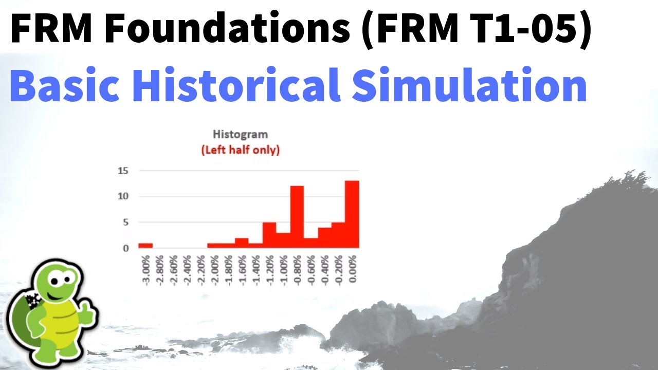
I'd like to show you the basic historical simulation approach to Value at Risk using the example that's been the frm for many years this is a simple idea we select a window we sort the returns from best to worst so that we can identify the lost tale we look down that sort of list for the lost quantile associated with our level of confidence then I'll add a level of sophistication and show you age weighted historical simulation aka hybrid because it's a hybrid between the historical simulation and the exponentially weighted moving average and here the ideas that returns that are more recent get greater weight but we still have a sorted list and then most of the viewers of this video can stop and go do something else unless you want to go to the end where I will show you technically the strict implementation of this age weighted historical simulation where we make another advanced sophisticated assumption about the data that we're looking at to show you historical simulation I've just used the data from Linda Allen's table 2. 3 that's in her chapter two and the reason I'm showing you this data is that it's assigned in the frm topic for part one and has been for over a decade that shows you how basic is this historical simulation and the idea here is really simple we need to just select a historical window how long will that window be and linda allen selects 100 days so the variable happens to be k and it equals 100 days there's a trade-off here normally we like as much data as possible but in the case of historical simulation more data means going back further in time so that's less recent data so we have a trade-off here between data and recency so she uses 100 days and then the idea with basic historical simulation is that we just sort the returns from worst to best so I've here at the top I have the worst return over the last 100 days and it's a negative as we might expect negative 3. 3 percent sometimes in risk value at risk we drop the negatives because we know we're in the lost tail I've retained them so the worst return is negative three point three percent as a daily return the second worst is negative two point nine percent and so on I'm also showing how many days periods or days ago that was so negative three point three percent was the daily return three days ago negative two point nine our second worst was two days ago negative two point seven with sixty-five days ago so it's more than half way back through our historical window but I'm not going to use the periods ago in the basic historical simulation because the idea here is we just sort the returns and really just look down that list to identify the quantile associated with our desired confidence level right so in these examples it's our hourly typical choice of a 95% confidence value trest which means we want to locate the quantile associated with the 5% tail now as a discrete distribution for better or worse the truth is there's three valid choices I think the best one is to follow Kevin Dowd here strictly speaking and in the case of the 95 percent bar that means counting down 1 2 3 4 5 to the sixth worst return obviously these are cumulative weights and that six worth return is negative two point three zero percent of course I'm not to focus on the weights here because that they're all each of these returns has the same weight of 1/100 because that's how many days are in this distribution I'm not showing the rest of the distribution so cumin if Li is also very straightforward so as a 95 percent var I retrieved the sixth worst return in formulaic ly that's just one minus our confidence level multiplied by the number of periods in our window or days and our window in this case and we do add one so that's in this case for a 95% VAR that's a 5% significance times 100 plus 1 equals the sixth worst return in our sorted list is the answer to the 95% var now I think that so that's the I think that's the best approach because it's assigned by coming down in the frm and also I happen to think it's intuitive because here I've just squared off the 5% tail right that's the worst tail of the distribution and then we're locating me return that's just adjacent right outside the tail as the VAR quantile I happen to think that's intuitive but I certainly understand if we just want to say if you want to just go 1 2 3 4 5 here is 5 and select the fifth worst return Jorian would do that and that's also a valid answer finally we could settle on the difference here so to speak and use the average or interpolation here of negative 2 point 3 5 the average of these two that's also a valid answer to the 95% bar 3 ways to go why are we stuck with the choice there again because of the discrete distribution if it were continuous we would not have to choose ok now we get a little more sophisticated with the age weighted historical simulation which has the synonym of hybrid and it's also called a hybrid Linda Allen calls it a hybrid historical simulation because it's hybrid between historical simulation and the weights are using the exponentially weighted moving average approach that we use that is popular for volatility so here the idea similar to historical simulation we're still going to sort the returns from worst to best and look at the tail however in basic historical simulation each of these returns implicitly got the same weight 100th or 1% was the way now with the age weighted circle simulation the more recent returns get greater weight and more distant returns get less weight and what is the logic well with there's lots of logics we can use but the exponentially weighted moving average is very elegant and efficient and here the idea is that the weight decline exponentially or the constant ratio between two days is always our lambda value in this case point nine eight so that means that if the return happened yesterday its weight would be 1 minus lambda in this case I've lambda point nine eight that means yesterday's weight would be two percent and then the day before that we would just multiply by lambda so that's what I mean by under exponentially weighted moving average the weights are in constant ratio to each other and that ratio is lambda so 1 minus lambda yesterday's wait day before that will be multiplied by lambda if we want to go back to three days ago we multiply lambda lambda again and so that's why the weight assigned to n days ago is given by 1 minus lambda x mile and is not so great lambda raised to the N minus 1 that's why this happens to be a formula that in the frm Canada's generally memorize right so if I want the wait 10 days ago its lambda race to the 10 minus 1 or lambda raised to the nine multiplied by 1 minus lambda so the only thing about that and that would be a fine way to get the weight the only thing about that is if we have a hundred days in our window here this is a formula for an infinite series so if we add them up we're going to come a little short of one percent or one hundred percent and so we can lever these up proportionally just by dividing this by that's my dove Division sign here by 1 minus lambda raised to the K power so that'll plus this up a little and then that will ensure that regardless of our window in this case it's a hundred days the summation of the weights will be exactly one hundred percent okay so you can look at a spreadsheet if you'd like to take a closer look there at the weighting function and but I'll just step back to conceptually here just to highlight the fact that now we can compare to the basic historical simulation and we saw that the worst return among the one the selected 100 day window was negative three point three percent which in a basic historical simulation gotta wait implicitly of one hundredth one percent here because it's only three days ago its weight is two point to one percent our second worst return of negative two point nine percent is very recent only two days ago it gets a two point two six percent way and then that third worst return sixty five days ago only gets a point six three percent so you see how this column in contrast to basic historical simulation is really the essence of this hybrid aka age weighted historical simulation approach and then now that cumulative simply adds them right the four point four seven is two point two one plus two point two six and we have a cumulative weighting that really x is more accelerated due to these worst returns being so recent and so it's fine at this point to stop even stop the video if you like and say that we can use this cumulative weighs human of approach here to the hybrid weights to ascertaining our 95% bar is somewhere around negative two point seven percent that's why I've highlighted this in yellow and you could just see in contrast that's how that's the answer somewhere around here we get under hybrid or age weighted as opposed to what we got when we not age wait we got only negative 2.
30 percent so that's a fine stopping point unless you want to go with me further and I'll just round out and explain the strict technical interpretation that Linda Allen uses in the book and that we know can be confusing and that is also in the spreadsheet I won't certainly won't go into greater detail but the key thing I do here is I take what we've already looked at here and insert I break these observations out and insert midpoints I'll show you why in a second and then we have mass centered weights associated with each of the observation returns and their midpoints and so the bottom line here is we're gonna we take it one more technical step and do mass centering and then interpolation we're gonna have a slightly different set of cumulative weights than we have what do we have it are here under maybe called this naive age weighted naive age weighted sophisticated age weighted and rather than go through those calculations what I have are just some diagrams to explain that logic and Linda Allen that we know from experience confuses almost every candidate that reads it the first time and what we have here is I've got the worst return that's familiar right negative three point three percent was the worst return and we've already established that because that was only three days ago that its age weighting is to point to one percent so here's the key confusing idea that Linda Allen assert inserts and that is that she treats this observation this negative 3. 30% as a random event where it's probability mass is centered on where it actually happened to be observed and so the weight of two point two 1% here then you can see is now a probability mass centered at the negative 3. 3% starting over here at a weight of zero because is the worst and going extending over here to the midpoint between that worst and second worst return you'll recall the second worst return was negative two point nine percent my scale is probably a little off here but the midpoint between our worst return and our second worst return is negative three point one right here and so because this observation is now considered to be a random event where the probability mass is centered on the observation it is the three point three return that we observed is considered to be associated with are aligned with the one point one one or a little rounded but half of the two point two one percent right so that's the idea fifty percent to the left and fifty percent to the right treats this as a random event so the three point three is associated with a wick human of weight of one point one and then we go out to the midpoint here of three point one and that's associated with the 2.
21 weight right so now keep going now I'll add here is our second worst return and aged waited it got a two point two six percent and again it's a random event centered at 50 percent goes to the left here to them that midpoint 50 percent goes to the right which is the midpoint between the second and third worst and happens to be negative two point eight percent so now the return of negative two point nine percent it is aligned cumulative ly with well the two point to one percent here plus half of this density which is around rounding Oh at one point one three actually not rounding so much and so you can see two point two one plus one point one three gets us to three point three four is the cumulative weight associated with this second worst return okay I'll keep going and now if we go out to the midpoint here between the second and third that is a midpoint observation negative two point eight it is associated with the cumulative weight that adds these two right to point two one plus two point two six is four point four seven another step and now we have the third worst observation negative return negative two point seven it only had a weight of negative I'm sorry of point six three and the two point seven then as a return is associated with right all of this four point four seven here plus half of this 0. 63 treating as a random variable and that this one is rounded it's about point two it's 0. 32 if we round it up so you can see half of that gets added and that's why this third worst return of negative two point seven is associated with a cumulative weight of four point seven nine and then finally this is my last one we extend the cumulative way all the way out to the midpoint between the third worst return of negative two point seven and what I'm not showing but what must be negative two point five the midpoint between the that's the third worst and this is the fourth worst the midpoint is negative two point six and so that as a midpoint observation is associated with a cumulative weight of five point one one because it's all three of these weights added together okay right so we've got the two point seven return goes to four point seven nine and the two point six goes to five point one one and then finally what Linda Allen does interpolate and you can see again we're looking for the five percent quantile you can see it's between four point seven nine to five point one one but it's going to be closer here to the right it's going to be close somewhere about here closer to the two point six and it ends up being exactly negative two point six three sorry negative two point six three is the interpolation between these two cumulative weights right look look interpolating at 5% finding that return between negative two point seven and negative 2.