Okay so last time we've talked about the spirit of the null hypothesis significance testing and this week we're going to actually play this game of null hypothesis significane testing with data so before we practice how to run this null hypothesis significance testing let's just start with talking about a research. So this one of the major risk factors for glaucoma is ocular hypertension and lowering the intraocular pressure is probably the only manageable and modifiable risk factor to slow the progression of this blinding disease and so the traditional first-line approach has been topical pharmacotherapy and there are quite a few options available. So among others a newer generation of drug called rho kinase inhibitors were compared against a popular beta blocker called timolol for its effectiveness and efficacy in a clinical trial started in 2014 and then they published their result in 2018.
So in their study, they recruited a group of patients with either diagnosed with the ocular hypertension or open-angle glaucoma and they measured the patient's unmedicated baseline intraocular pressure before the researchers assigned them to the respective treatment groups. They measured patients' intraocular pressures with Goldmann and after that, they split the group of patients into three different treatment groups and here a baseline sample statistics of intraocular pressures for one group where the number of patients was 206 and the mean intraocular pressure was 23. 51 millimetre mercury with a standard deviation of 1.
654 millimetre mercury. So according to the college of optometrists and the cutoff of untreated intraocular pressure or ocular hypertension is at 21 millimetre mercury and over with Goldman when the IOP is measured with the Goldmann tonometry. So then the question is "are the patient's average intraocular pressure in the previous study for that specific group statistically above the cutoff guideline of the college of optometrists?
" Of course the number looks larger than the cutoff but how do we know so you want to make sure that you know if it is just a specific to the sample or not because this is only the single sample you have but what if you have different value with the different samples right so understandably every sample will give you different statistics then how do we know and from this sample statistics is actually representing the population patient IOP so that we can say this is definitely greater than the cutoff value or not. So that's exactly the reason why and where we need the central limit theorem, if you still remember, from the last lecture. So the central limit theorem is the connecting theorem between the sample and population so this is kind of a bridging theory that we can actually use our sample to say something about the population something about how close or far away our sample means in estimating the population mean by taking account into the sampling variation.
So now we are ready to play the game of null hypothesis significance testing. So to play this game of null hypothesis significance testing, we need to identify and state the practical question that is in need of a statistical testing. So the question I see from the study is the following.
On average is the patient's intraocular pressure greater than 21 millimetre mercury just to make sure that they meet the criteria so that they are indeed abnormal in terms of intraocular pressure so, in this case, the parameter of interest so you need to identify the parameter to be tested which is the population mean intraocular pressure of the ocular hypertension patients. That is the population average intraocular pressure of all the ocular hypertensive patients. So the population parameter is represented by the greek letter mu.
So from this question now we can turn this question into a pair of null and the alternative hypothesis where the null represents the status quo. So we're going to say the population mean intraocular pressure will not be different from 21 millimetre mercury or more or less same as 21 millimetre mercury. On the other hand, our alternative will be opposite to the null where it will say no it will be different from 21 millimetre mercury.
But more specifically in this case we don't care about the value less than 21 millimeter mercury so it should be bigger than the cutoff value so our sample mean should be bigger than the 21 millimetre mercury so that's what we care in this question and once we have the pair of hypotheses then we need to have a decision rule in place before we see the data. Well of course we already have the data but let's pretend that we did not see them yet. But as a general rule, you cannot have this decision rule after you see the data.
So you can think of it as kind of a live betting or playing lottery and you must place your bet before the match starts because you cannot place your bet after everything is said and done. Otherwise, it's known as cheating. So now you're ready to recruit the patients after you're setting the decision rule and measure the outcome variable which in this case patient's intraocular pressures to test your hypothesis.
Well we already have our sample statistics so we can estimate the location of the parameter and express our uncertainty of the estimate. But then, how do we do that? That is the question.
So remember this equation? So this equation provides the one-sample z test statistics to test a certain population mean which is in this case mu zero so that is some sort of testing value so this is testing value against a sample mean so sample mean so we assume that this sample mean is coming from this population and then we want to see how far this sample mean is compared to this cutoff value basically in our case. But this z-test can only be used when you know the population mean and the standard deviation.
Remember that this one, this actually represents the population standard deviation but in practice, it is almost always the case that we do not have that information and if we know the information about the population then why do we ever bother to actually take the sample and then try to infer something about the population? when we already know about the population right? So in many cases, we do not know the population standard deviation so instead what we do is to replace this population standard deviation with the sample standard deviation.
But if we do that, so that actually becomes then the t-test. Now the z is actually normally distributed but the t distribution is not normally distributed even though it looks pretty similar to the normal distribution. So when this you know the population standard deviation is replaced with the sample standard deviation then the resulting statistics does not follow a normal distribution anymore.
So here the one sample t statistics has the t distribution with the n minus one degrees of freedom so that is degrees of freedom n minus one so here the n represents the size of the sample right so we need to take away one because we are testing the mean so the t statistics uses sample mean which is fixed for the sample. However you can change or you can have a different sample members except for the last one that's why we take away one because there's only one fixed statistics used to calculate the t statistics right so that is basically the same as the standard deviation so there's a degrees of freedom and as a function of degrees of freedom, the shape of the t distribution actually changes so what we're seeing here in the graph are the four different t distributions with different degrees of freedom so I don't know if you still remember it but you know this is a ni right or nu in Greek if this is not v, another notation for degrees of freedom so this is the same as degrees of freedom. The yellow colour represents the t distribution with a sample size of two, the sample size of two because degrees of freedom for the t distribution is n minus one.
So that means the sample size for this distribution is two right two minus one is one but that's what it is so if you look at the yellow curve and the black curve right the black curve here is actually having the infinite number of degrees of freedom which is basically the normal distribution so if you increase the sample size then the t distribution actually converges to a normal distribution and if you compare this a yellow one right and with the black one you can see that the tail, both tails of the yellow distribution is actually thicker compared to the normal distribution by this much. So effectively that'll actually make the yellow curve looks thinner at the centre compared to the normal distribution which is the black one so that is called the leptokurtic. So it looks lean and leaner than the ideal normal distribution but it becomes more look like a normal distribution as the sample size increases.
Okay so now we can calculate the t statistics and as we have all the statistics we need, so we can just then use the t equation. It's very simple so t degrees of freedom equals x bar minus mu 0 and sd over square root of n so. .
. t so 206 minus one so the degrees of freedom equals x bar is 23. 51 and our cutoff intraocular pressure was 21 right and then sd is 1.
654 over square root of 206 right so then that is in the numerator is 2. 51 and now we need a calculator there we go so we need one point. .
. Okay so this is the standard error of the mean so that's the denominator however. .
. there we go five all right so and that's Okay so that is 21. 83 was it yep uh yep rounded to two decimal places so that is our t value so t 205 21.
83 so what that means is that so what we just did is to standardise our sample mean to the sampling distribution of the t statistics with the degrees of freedom of 205. So the size of our t statistics is telling us how far it is from the centre of the sampling distribution which is 21, 21 millimetre mercury right now then how do we make the decision if this t value is statistically greater than the cutoff value? So what you're going to do in practice is that you will compare the likelihood of observing this statistics under the null distribution against the preset likelihood which is the decision rule you would have set in place before you calculated this t statistics so this preset likelihood is called the level of significance alpha and it is typically set at 0.
05 so 0. 05 which is the area under any sampling distribution representing the likelihood of observing a critical statistics or more extreme so that's what that means. So let's say this is the standardised sampling distribution of t with the degrees of freedom of 205 right representing the null distribution centred around 21 millimetre mercury so now this zero represents the cut-off value right so this is a sampling distribution centred around the cut-off value 21 millilitre mercury but now this is a standardised so that mean that cutoff is now mean and that it is shifted to.
. . so that 21 millimetre mercury is standardised to be located at zero in the t space okay so that's what just happens so that that's what the sampling distribution represents here so we want to determine if our test statistics is bigger than this cutoff.
So well obviously we know that our t statistics was bigger than zero because it was 21. 83 so it must be somewhere about like here right but you know there should be a rule to be set to say that say hands down that our sample statistics is statistically bigger. So for example if the test statistics is located right next to say and to the mean right then the likelihood that we see this statistics at this location or more extreme is almost 50 so the exact probability they will see this statistics is actually found on this curve right but you want to consider other extreme cases because this is only the single sample but in calculating the probability you need to consider other possibilities that samples can be more extreme than this.
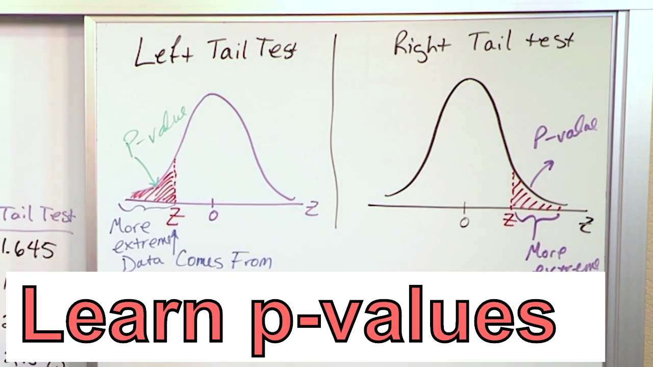
This way right and you just basically add all these probabilities up to the right tail end. It becomes the area under the curve right so that area under the curve the meaning of it is that the likelihood that you will see a certain statistics say this one or more extreme this way but that is the meaning of the area under the curve summed probability right and then this is actually the the definition of p-value of your statistics how likely are you going to see the statistics or more extreme statistics right when your sample statistics actually fall here but you know we'll talk about this later on but when your sample statistics fall here then the likelihood that this will happen is almost 50% right meaning that every other time you will see the statistics happen just by sheer chance so the patient group may be the real patient 50 of time but other times even normals can be this high so you want to move this kind of boundary further to this way right so that you and also other people think that the statistics does not come by very often right. So now the question becomes then where you draw a line to determine how far out it should be from the centre so you basically need another cutoff value beyond which your statistics needs to be, to say that this much difference is very unlikely to be seen just by chance and that cut off is called the critical statistics and that is somewhere out in the tail end so let's erase this and somewhere out here we have t-critical value so this is a line where your statistics need to go beyond to say that your statistics is statistically significantly different from no difference okay so that represents no difference basically so whatever the value you want to compare this was 21 millimetre mercury before right but it can be any value right but you know this t distribution is just normalised against whatever value you try to compare so that's what that means so that's t critical so that is the cutoff value right to determine if your statistics is significant or not and then that t critical statistics happens to be the boundary beyond which the area under the curve becomes 0.
05 or by convention. It doesn't have to be always 5% but that is the number people pretty much always use and unless otherwise noted differently. So this is the t crit that's a t critical value and this is the boundary beyond which area the curve the right tail end to the infinity it this becomes 0.
05 and this is what is called level of significance. This is another summed probability under a sampling distribution. So that is supposed to be determined before we collect the data.
So you can just assume that your decision rule is almost always alpha 0. 05 to decide if your statistics is statistically significant or not and now how do we calculate this area under the curve and the critical statistics? We can do this easily with any statistical software.
So let's just find out the t the critical statistics beyond which the area that curve becomes alpha 0. 05 with Jamovi. Okay if you haven't done so now is the time to open Jamovi excuse me and make sure that you have installed the distraction module right and I showed you how to install the distraction module by clicking this plus sign and you go to Jamovi library to find out the distraction module and you can just you know click install then it'll automatically install the distraction module and so to find out the area under the curve at any critical statistics you can use this distraction module so now this time we're not dealing with normal distribution now the distribution we're dealing with is the t distribution so you have to click t distribution so now we have the input parameters so you need to enter the degrees of freedom so what the Jamovi is showing you is actually the t distribution with the degrees of freedom of one so that means sample size two and lambda the lambda here the greek letter lambda here is the centre value so that is just the location parameter basically so this is zeros we don't have to change it but we have to change the degrees of freedom to 205 right so that was the degrees of freedom for our sample and if you do that see that looks more like a normal distribution so from here because we do not know the actual critical statistics beyond which there and the curve becomes 0.
05 so we do not use this function okay because to be able to calculate the probability then you should be able to know where is the cutoff value right and or the boundary value to calculate that probability so this is inverse process where we need to find the critical statistics on here right on the axis of t values where it becomes 0. 05 so and you just to compute quantiles and the p-value becomes 0. 05 okay and this as I said the area under the curve represents cumulative, the summed probability So this is giving you, so by convention when you calculate the cumulative distribution, the area under the curve it always starts from the negative infinity up to a certain point right so that's what this distraction module is doing it's adding all the probabilities from the negative infinity up to this critical statistics, which is a negative 1.
652 so up until that critical statistics the area under the curve here will become 0. 05 so that's what it is right but this is not the tail end that we want to calculate the area under the curve it is actually this side right but if you think about the property of the t distribution it is perfectly symmetrical about the centre so and you can just to flip this over to here and it's going to be just mirror symmetry right so the t critical value here is a negative 1. 65 so and the positive 1.
652 and beyond will give you the exactly same alpha 0. 05 or the p 0. 05 basically or if you want to calculate the other side of the critical statistics then what you can do is to 1 minus this p-value so that becomes 0.
95 right and that is the other side of the t critical statistics which is exactly the same right the 1. 652 but we have just different sign but what it just calculated is the area under the curve from the negative infinity to this point right so the end of the curve below this t statistics will become 95% So what that means is that the remaining right tail end will be 0. 05 so this is another way to find the t critical statistics using this distraction module and finally we can calculate the p-value which is the summed probability of observing the sample statistics as big as the one we have or more extreme so, in this case, our sample statistics becomes the boundary to calculate the area under the curve which is the p-value of the statistics so this is the same as the level of significance.
The only difference is that you can only calculate the p-value after you know your sample statistics whereas the alpha . 05 is preset and you know regardless of your sample data it is always 0. 05 so let's say here is the critical statistics right where beyond which the area under the curve becomes 0.
05 right so this is already given even before you look at the data but the p-value is the probability that you will see your data or more extreme. So say if your statistics falls outside so that is t_test that is your sample statistics then the p-value becomes so. .
. this becomes the boundary of the p-value right but this is the p value okay so if your data falls below the t crit here that is another sample statistics t test all right then the probability that you will see this statistics here and more extreme will become this area under the curve P prime. okay so that is the definition of the p-value and now if we so how do we calculate the p-value again we can just go back to Jamovi and just enter this you know test the statistics to find out the area under the curve right so in this case, we know the boundary so all we have to do is to find out the cumulative probability using this t statistics as a boundary value so if I just.
. . So this is our previous Jamovi so now we don't have to change here anything here because it's all the same.
Now instead of a compute quantiles you need to calculate the probability and we know the cutoff value so that this time the cutoff value becomes our test statistics I think it was 21. 83 right so let me see was I think it was right so now let's just do this and the probability is well it is not exactly zero but it is close to zero so if you look at the tick marks here only goes up to four and our statistics is 21. 83 so it is somewhere out here right which is a very very tiny tiny right tail end so the likelihood that you will see this t statistics or more extreme is really really small it is highly highly unlikely to see this size of the t statistics okay so now we can make the decision about the null you may find it very strange to make a decision this way but it is all about the null as the name of the game suggests the null hypothesis significance testing so there are only two decisions you either reject the null or fail to reject the null okay?
Depending upon who you ask some people will accept either null or the alternative hypothesis but because of the historical reason and we'll just stick to this decision making. so you either reject the null or to fail to reject the null okay based on the following criteria. So when you are comparing the p value against alpha so you're basically comparing two probabilities right alpha is preset probability and p-value is the probability of your statistics right so if the p-value is less than alpha 0.
05. So it is pretty much given unless it is specifically noted that they used a different value but implicitly it is almost always alpha . 05 you compare your p value against alpha and if it is less than alpha 0.
05 you can reject the null okay reject the null of no difference. On the other hand if the p-value is greater than or equal to the alpha 0. 05 then you just fail to reject the null of no difference right so in our case our p-value of that the intraocular pressure right to see that t value of 21.
83 is practically zero it is a very very small it is obviously smaller than alpha 0. 05 so that means we reject the null of the no difference and we can conclude that we have enough evidence to support our alternative hypothesis, which is that the patient's intraocular pressure on average is greater than the cut-off value of 21 millimetre mercury. So this is one way to make a decision okay so you compare two probabilities and if the probability that you will see your statistics is less than the preset alpha 0.
05 then you reject the null of no difference and you have strong enough evidence to support your alternative hypothesis which is typically your research question. You can use statistics to make the same decision to arrive the same decision so the t statistics right in this case we have t statistics if your t statistics is greater than critical statistics right then you can reject the null otherwise you fail to reject the null so in this case our statistics this was 21. 83 and our critical statistics was 1.
652 right so because our test statistics sample statistics is greater than the critical statistics so we reject the null. In fact these two are related right so you can only calculate the p value based on the sample statistics because that you know that your test statistics becomes the boundary to calculate the p value and alpha is the same thing you can only calculate alpha when you know the critical statistics so whichever criteria you use really doesn't matter but the most preferred way to make the decision is to compare two probabilities so you compare p against alpha so that's because alpha 0. 05 is almost never changed.
On the other hand t critical statistics, the critical statistics always change according to the sample size. So you have to calculate the critical statistics for different samples. However you don't have to change your alpha because it is pretty much always almost always 0.
05. So the preferred way to make the decision is to compare two probabilities so p against alpha so if this is just too complicated to make a decision then you all and all you have to remember is to compare p against alpha 0. 05 if the p value is less than alpha 0.
05 then you reject the null and you have strong evidence to support your alternative hypothesis that's all there is to it. Otherwise you just fail to reject the null and you do not have strong enough evidence to support your alternative hypothesis which is typically your research hypothesis. Now let's rewind what we have done and we start from the beginning.
So first in playing the game of null hypothesis significance testing you first need to state the practical question that you want to test by statistics so it did so the question here is the on average is the patient's IOP greater than 21 millimetre mercury. So we just want to make sure that they, as a group, have indeed higher than normal intraocular pressure. So the next step is to identify the parameter of interest which is the population mean, IOP of the ocular hypertensive patients which is the outcome measure of the study.
So from this research question now you convert the research question into a pair of a null and the alternative hypothesis where the null represents the status quo saying the population mean intracoular pressure will not be different from the cutoff. On the other hand our alternative will be that the average IOP of the patients will be bigger than the cut-off value which is what we expect to see. So once we have the pair of hypotheses then we need to have a decision rule in place before we see the data and the decision rule was of 0.
05 right alpha 0. 05 so your decision rule will be that if the p value the likelihood that you will see the test statistics is less than this value okay and you will reject the null otherwise you fail to reject the null, that's all there is to it so you use this alpha . 05 as your criteria.
Now you're ready to collect the data calculate the statistics and the p value to test the hypothesis and it turned out to be this so t degrees of freedom plus 21. 83 and the p value even though we weren't able to look at the exact value what you can say is that less than . 05 okay so this way we know that the p-value I mean all we know is that p-value is very close to zero.
I'm pretty sure that it is less than 0. 00001 but all that matters is that the p-value is just less than alpha 0. 05 to reject null so that's all that matters so now we can make the decision so as the p-value is less than of a 0.
05 we reject the null right we reject we reject the null and we say that the patient's intraocular pressure on average are indeed higher than the cutoff value of 21 millimetre mercury and that is basically our final conclusion of the null hypothesis significance testing so the previous hypothesis testing is called a directional or one-tailed testing because our alternative hypothesis was concerned about the direction of the difference which was made explicit in the alternative hypothesis. However you don't always have to make clear prediction about the direction of the difference because it is not always the case you know the expected direction of the outcome. So when you are setting up a pair of hypotheses and null is always stated as there will be no effect no change or no difference between the values being compared so you do not implicate the direction when you're setting up a null hypothesis, that is because what you're saying is that basically they are the same right your sample mean will be same as the value that being compared so you do not implicate the direction the expected direction of the outcome in the null but you can implicate the direction of the difference in the alternative hypothesis like in the previous example so this is what we did so when you so in this in our previous case we expected that the patient's average IOP is greater than 21 right so in this case then you expect to see your t statistics to be positive right so this is zero so centre is zero difference basically and then the positive side the right side is the positive side and you expect your t statistics fall on this positive side somewhere here right and then the p value that you will see this statistics or more extreme this way is this area under the curve okay so that's the p value so that's the p that the t statistics this location or more extreme values will be found so that is a summed probability so that is definition of p-value in case your alternative hypothesis is this so you expect your sample mean to be greater than certain value so your t should be positive in this case but you can have the opposite alternative hypothesis opposite directional hypothesis in that you expect your sample mean to be smaller than a certain value.
So in this case then you expect your t statistics to be negative so that's negative t and your p value will be the area under the curve bound by your statistics and to the left side of the curve. Because this is a zero difference, going further away from the centre actually represents more extreme values. So if you expect your sample mean to be less than some value and the likelihood that you will see this t negative statistics or more extreme is the area under the curve bound by your statistics and to the left side so that is your p here right so if you do this, rearrange this then you move this to this side and you're going to take away see?
so this difference should be positive that's why your statistics to be on the right side and the same thing, you just rearrange this move to the left side mu zero becomes zero so this difference now should be negative right so when you look at your t statistics you have to actually look at the sign carefully to make sure that if your statistics in the right direction as in the expected direction, especially for the one-tailed hypothesis. But it is not always the case you know the direction of the difference and you don't have to. So if the direction of the difference does not matter or you're not sure about the direction of the expected outcome then you can make your alternative hypothesis two-tailed or two-sided this way so now you place your bet on both sides right and you don't know actually where your t statistics will fall either to the left or to the right you don't know but you know wherever it falls as long as it falls beyond one of these t's, negative t for this t then you will say that your sample mean is different from the certain value, specified value here.
So if you rearrange this this is a mu minus mu zero is not equal to zero right so it doesn't matter which way it is different from zero. It can be negative or positive so you can go both ways so now you have to consider this side and this side together so that's why the p-value becomes doubled. Right because you're considering the both sides and these two vertical sign around the t small t means so that is that absolute value so that t means either negative t or t so this two vertical bars actually removes the sign from any value right so it only takes account into the size of the value, only the size so if you just do this if I say 2 then it's either negative 2 or two okay so that's what that the absolute sign means.
Now then let's look at some example to run the two-tailed hypothesis. So let's assume that you are running a practice in Glasgow. You hired a new eye care professional to run an exam for you and fit the glasses for the clients while you're focusing on running the practice.
After a while, you're getting complaints from the clients that they cannot see well with their prescribed specs. So as an eye care professional yourself, now you're wondering if your clients are properly corrected to six six vision so you give calls to a random clients and bring them back to test their best-corrected visual acuity in logMAR. Of course, you're hoping that the clients are corrected to zero logMAR by default but your hypothesis is that no they're not.
So let's play this game of the null hypothesis significance testing again step by step. First you need to state the practical question that is in need of statistical testing which in this case on average is the patient's BCVA, the best-corrected visual acuity, logMAR of 0. 0 so that is the question you have and you want to actually test it formally with the null hypothesis significance testing.
So the parameter of interest is the population mean BCVA which is the outcome measure of your study and from this question we convert the research question into a pair of a null and an alternative hypothesis where the null represents this the status quo saying that the population mean BCVA should be the logMAR of zero right or not be different from the testing value. On the other hand, our alternative will be that the average visual acuity average BCVA of the clients will be different from the testing value which in this case the direction does not really matter much because our goal is to show if they are statistically different from the logMAR of 0. 0 in any direction right in case of myopes if it is less than zero then the clients are overcorrected whereas if it is more than zero then the clients are undercorrected, so just to simply speaking.
So either way it goes it's not optimal, so they're not optimally corrected. So now we have this pair of hypothesis then now we need to have a decision rule in place before we collect the data and the decision rule is again you know it's almost always alpha 0. 05.
So we will test our hypothesis using this level of significance alpha 0. 05. So now here we have the collected data from the 16 clients.
so. . .
you need to calculate the statistics and P value and this is what we obtained from the clients and we have 16 clients and you calculated the average BCVA and it turned out to be 0. 05 logMAR with a standard deviation of 0. 0816.
So there's only 0. 05 difference from the optimal 0. 0 logMAR but given the standard deviation, given the sampling variation we'd like to know if this is statistically different from logMAR of 0.
0. So now you should calculate the t statistics. So the t in this case and the degrees of freedom is 16 minus 1 equals so and the mean sample mean is five and we're just comparing this against zero and the standard deviation is 0.
0816 equal over square root of 16. So that's how we calculate the t statistics. Now the numerator is just 0.
05 and this 4 right because square root of 16 is 4. That is 0. 05 over 0.
04 no 2. 204. Now I need a calculator.
So our t statistics is this value 2. 451 right so excuse me now we need to calculate the p value so the likelihood that we will see this much t value or more extreme so p equals what now let's calculate the p value with Jamovi but before we do that so once we have the p value then we can compare our p value against alpha right so that was the decision rule. So you either reject or fail to reject the null depending upon your p-value against alpha so but before we do that let me explain how the level of significance is actually placed in two-tailed testing.
So here the level of significance alpha is still 0. 05 but in case of two-tailed testing you split the level of significance alpha 0. 05 into halves and place them in both tails okay so somewhere here and each area under the curve should be 0.
025 0. 025 so when you add them together it becomes alpha 0. 05 so because this is a two-tailed you have to split this probability into two halves and into both tail ends okay so that now the effectively the area under the curve to be compared against actually shrunk by half right and because you have two areas under the curve, accordingly there should be two critical boundaries beyond which area under the curve should be 0.
025 each. So this is where you need Jamovi to find these two critical values as you can see so one value should be the negative somewhere here and that is the t corresponds to the left 0. 025 right and that one is somewhere here positive right but by convention I told you that it is actually 97.
5th percentile right from the left. So let's just use Jamovi to find out these two critical values. Okay so here is our Jamovi and to find out those two critical values, you need this distraction module and because we're dealing with the t distribution you choose t distribution now because the degrees of freedom is 15 you just type in 15 and you want to find out the quantile that is corresponding to this area under the curve which is 0.
025 right but what we need is a cumulative quantile from the left up to the critical point so you need to choose this one and then here we have the left side critical value so up until negative 2. 131 from all the way to negative to this point, the area under the curve will be 0. 025 and because we know that the t distribution is a mirror symmetry then the other cutoff will be the x2 will be positive 2.
131 right so it in fact the well what's the value sorry and three one So we have two critical values now two one three one all right so two one three one is about here so that's the left t_crit t_. 025 size and that means the curve becomes oops alpha over two . 025 so that is negative 2.
131and here's another critical value. that's t it's actually 97. 5 percentile which is positive 2.
131 okay and this is another half alpha over two okay now where is then our statistics? By the way for the t distribution with the degrees of freedom of 15, the middle part here is now 95 percent and this range here that is the 95 confidence interval for the null hypothesis okay and now our statistics t statistics was 2. 548 no 2.
451 so 2. 451 is where? It's about here right so it is actually the t statistics is greater than this value so what that means is that this is actually statistically significant right but let's just do the p-value so p-value is actually the area under the curve bound by this to the right side okay now this p-value is less than alpha half of this alpha right 0.
025 so that means our statistics is statistically significant so let's just calculate this p value what is the exact p value here when the t(15) is 2. 451 okay so let's just then go back to Jamovi and now we need to use this right because we know the cutoff value and that is 2. 451 and calculate the probability that you will see the statistic more extreme okay so that is the p-value our p-value bound by our own statistics of 2.
451 and the p-value here this is a one-tailed p-value right but if you want to calculate the two two-tailed p-value you just basically multiply two by this probability then you will have the two-tailed probability which is a 0. 026 right but you can still compare this p-value against the right side of the alpha 0. 025 and still this p-value is less than the alpha 0.
025 right? So that means you reject the null of no difference and now you have strong evidence that the clients, the correction is not done correctly properly right and then you know that because this difference was positive right so actually they are undercorrected assuming that they're myopes right so that is the final conclusion of this study that you know that hired eye care professional actually messed up in fitting the glasses of the clients. So that is the morale of the story.