Lecture 6 - Regulatory Circuitry - MLCB24

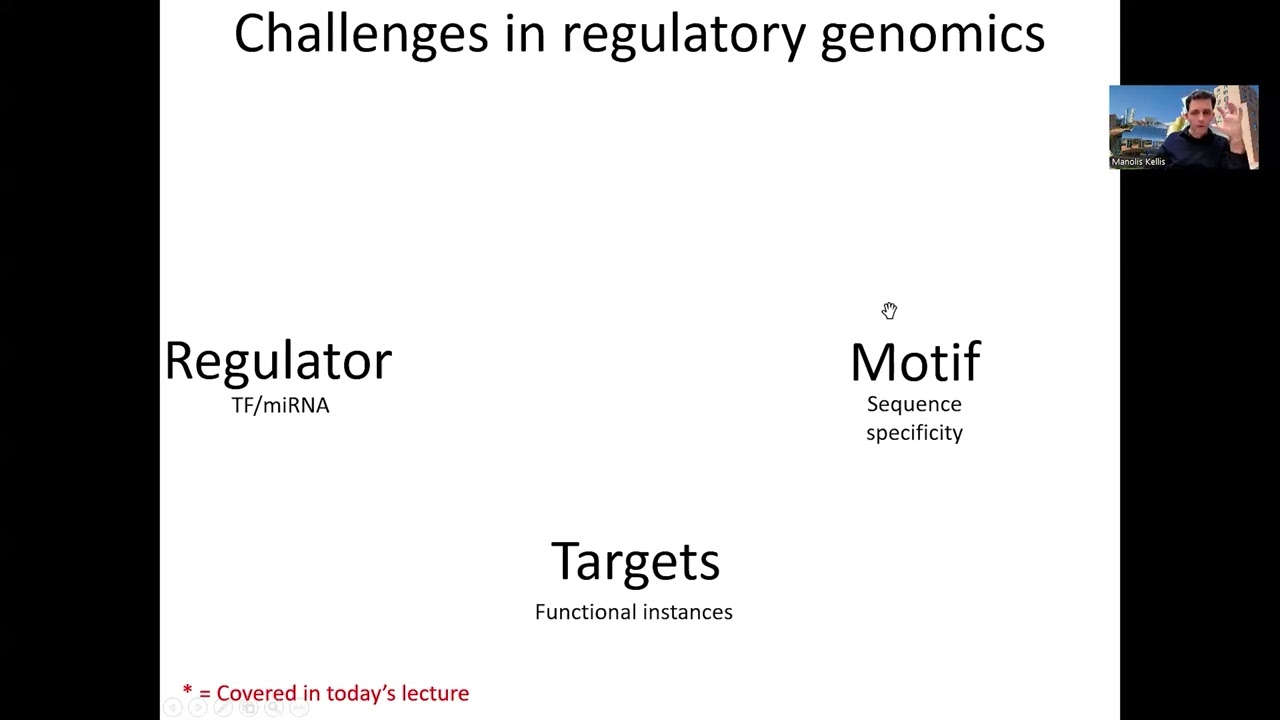
Al righty welcome everyone um so uh today we're going to be talking about regulatory circuitry so um we talked a lot about sort of how do we uh put together all these different pieces of the genome so um as I mentioned earlier 93% of disease Associated genetic variants that are causal for disease are in fact not found in protein coding regions instead they're found in non-coding Regions so the question is where are they are they hitting promoter regions enhancer regions other regions and if they are hitting enhancers what are their target genes what are their

Upstream Regulators what are the motifs that are recognized by these Regulators what are the Dynamics of these control regions across different cell types so these are a lot of the questions that we're going to be asking today about regulatory circuitry So today we're Focusing on the Foundations at the genomic level and then on Thursday we're going to be talking about networks that arise from these circuits and how do we understand biological networks so again a lot of stuff on the menu today we're going to be talking about epigenomic Dynamics and how do we learn chromatin

States across multiple cell types building on what we talked about last time to sort of understand how we can use this to understand the Dynamics of Gene regulation number two we're going to be looking at uh enhancer Gene linking so basically finding out which enhancers are targeted to what genes and also um what are the different methods that we can do that that we can use to to do that so we're going to be looking at three-dimensional genome confirmation we're going to be looking at correlation based methods and we're going to allude a little bit

to expression quantitative Trait lowai or eqtls which which are genetic variants that impact nearby gene expression rather than impact phenotypic traits so these are quantitative traits namely measuring something quantitative like expression but they are affecting not something at the organismal level instead something at the molecular level so we're going to be talking a lot more about etls at the genetics lectures which are going to be around lecture 17 Or so then we're going to look at how do we cover these words these regulatory motifs and we're going to look at enrichment expectation maximization G sampling

and also deep learning convolutional neural networks for motive Discovery then we're going to look at methods for Global motive Discovery using comparative genomics and for instance identification in the same way and then if time permits which it most likely will not we're Going to look at um massively parallel reporter assays for discovering this used to know everybody excited awesome I certainly am let's do it so uh here we are we're basically in the you know La last week of module one they're going to switch to protein structure then chemistry and then electronic health records and

so so forth and we've talked about expression we've talked about single cell we've talked about sequential data in her Mark of models We've talked about EP genomics and today we're talking about regulatory genomics but we're going to be building of course uh on all of the previous stuff and then next time we're going to be talking about networks so let's review a little bit h mark of models that we talked about last Thursday and uh how we actually can learn with them okay so again part of Gene regulation is understanding epigenomics because that's what gives

us The regulatory control regions like enhancers and promoters where the motifs themselves are sitting and where the enhancers are bound by different Regulators linking them to their target gen so basically a lot of the circuitry is physically instantiated there's physical links in the Genome of regulators binding DNA and DNA looping around to bind promoters and RNA polymer is binding to create uh you know the elongation and the transcription of the Rnas and so on so forth okay so there's a physical basis of these networks and last time we talked about the challenge of mapping hundreds

of millions of short reads to the genome very very fast we looked at the burs wheer transform implemented initially in Bai in B informatics that basically starts by adding a letter to Growing suffixes of a search string and then narrowing down the beam of searching by playing with these pointers that we Talked about we talked about how we can use this in multiple independent marks to start looking at each of these signals and how we can combine the signals together using hidden Mark of models which is what we're going to be focusing on at the

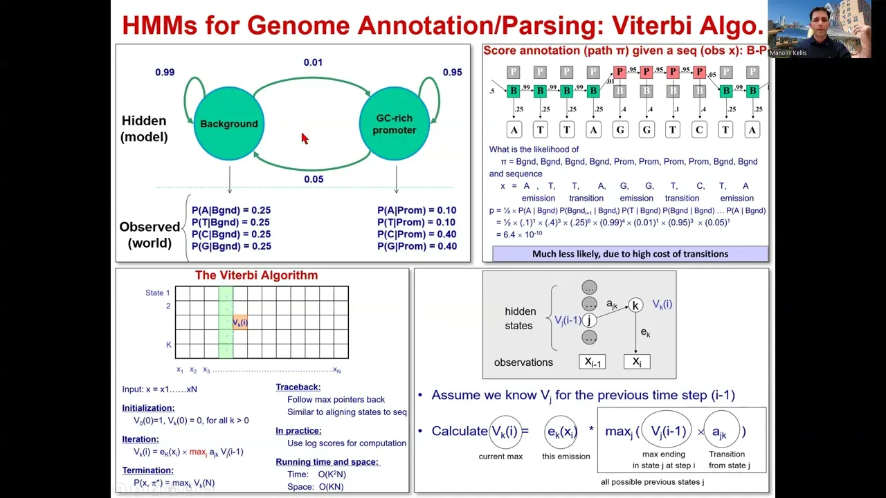
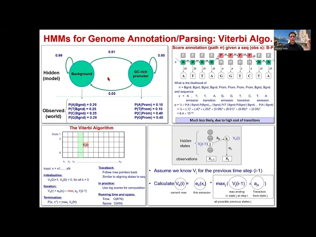
beginning of the lecture today and how these very powerful Paradigm of observed versus hidden can basically be applied with arrows between the hidden states to capture the dependencies Between different positions along the genome and this is Central because you're more likely to find say an enhancer region near a transcribed region than outside in in the middle of a bunch of repressed regions is everybody with me here so this relationships were encoded in the transition probability Matrix of hiden Mark of models that told us what is the probability that the next state at position I is

L given that the previous State at position I minus one was K and that gives us the K to L transition for example enhancer to promoter promoter to transcribe Etc and then the emissions where the probability of observing the I character in our string and this is the observe string given that the I state is K okay so that's the probability of emitting a particular character given our generative model everybody with me here so far and then we looked at the foundations For H Mar of models basically how do we transition between different states how

do we self transition to stay in the same state and that has implications for the length of either let's say promoter sequences or background sequences why does it have such implications because the probability of staying in the same state might be 99% but it decreases geometrically at every time step so basically if you look at blank sequence then the length distribution that you Would expect is actually a geometric length distribution for these states is everybody with me here now this is just the transition probabilities then there's the emission probabilities that basically tell us that from

some states are more likely to emit given characters for example acgt at equal probability with background but CNG at higher probability in a promoter State and then we saw how we can actually parse all of that by saying That the all promoter or all background sequences had some probabilities but that parsing this as background and then this as promoter and this as background was paying this 0.01 very low probability therefore paying a penalty of 100 if you wish for transitioning to only gain a marginal increase of less than two fold in the emission probability of

each of these characters okay so you know for four characters I would gain or let's say for Three characters I would gain roughly two fold and for one of them I would lose roughly two fold but I would pay 100 fold to get these incremental gains everybody with me here so therefore that transitioning in and out was actually very unlikely which is the whole point of H marov models the fact that you don't want to be very jittery in switching between different states instead you want to have some hyic some kind of damping of these

transition Probability so that you can kind of Leverage nearby positions to infer the probability of a given State given a given observation at a given time Point can I get a 543 to1 so how well you're following so far also lots of fives this is great unforced all right then we saw how yes we could score every single possible parts we could score every one of the exponential number of parses why exponential because at every Position I have two choices either here or here either here or here either here or here to the N length

so two to the N which is you know exponential um but I can find the optimal pars used dynamic programming how by setting up a variable the V variable that I would compute at every position assuming that I already knew the maximum score at every previous state and then the score the maximum possible score at that position would be a choice of one of the Maximum scores of the previous ones and the transition from that state to this statee so if I have a very high score in the previous state but I pay a very

high transition cost I will not want that if I have a very low score and I pay a relatively modest transition cost I don't want that either but if I have a high score and a high and a low transition cost then I'm doing great everybody with me here so that allowed me to Now update the next best Choice and remember the choice that led to it remember the arrow just like we did for dynamic programming alignment so by remembering these arrows when I arrive at the last column I choose the maximum one and then

I trace back my choices to restore the entire path and therefore the entire pars everybody with me here good and this was the the actual equation of the current maximum will be the emission penalty times the maximum Of this coupled choice of choosing the best previous one as long as the transition is not too costly okay so it's the product of the previous maximum and the transition any questions so far 543 to1 who's with me so far nice great all right so um this was the best single path so this is the best parse what's

a parse a parse is an interpretation of the Hidden State path that gave the series of Observations X okay so there's a hidden State Pi there's observations X and I infer the best such hidden state but this hidden state was one particular path one particular PA now if I care about a given position the amount of the probability mass that is concentrated in the best possible path the best possible pars is actually quite small there's many many many many paths An exponential number that can parse that entire sequence and there's a huge number of paths

that go through a given State at a given position the maximum likelihood path might be going through let's say the hidden state enhancer but there might be a hundred other paths rank number 2 3 4 5 all the way to 101 that basically go through the promoter State at that position so if I Care about the parse at a given position I could basically say let me take the best path overall and then look at what position is that path that single path going through in position 523 or I could say say well how about

I sum over all possible paths going through position through enhancer at position 523 and the sum of all possible paths going through position through State promoter at position 523 who's with me so far yes awesome so basically what I'm doing is that I'm adding up all possible paths going through b and exiting of course making it all the way to the end and then I'm comparing that total probability to the total probability of all possible paths going through P Instead at position 523 good 543 to1 who's with me on the question perfect beautiful all right

now the question is how do we calculate that Well I can calculate the total probability Mass going all the way to a point to a state at a given position by changing this maximum that we had before into a sum and therefore I am summing up over all the entire probability of all the possible paths why because if I have the total probability all the way to here and total probability all the way to there I can just add them up and get the total Probability all the way to there by recursion if I calculate

that variable now I can just sum it up to calculate the next one okay so just by calculating this change here as long as the previous one was the total probability sum all the way to the previous state then calculating the next one can just be done by also factoring in the transition probability and the emission probability and that gives me the total probability Mass all the way To the next point and therefore by iteration all the way to this point by recursion everybody with me here awesome now that gives me the entire probability Mass

going all the way to here but what about the one exiting well this was the forward algorithm that basically calculates the entire probability Mass all the way back to a given point and then the backward algorithm does the same thing but backwards okay very creatively named so we basically have The forward algorithm that I'm adding up to that point and the backward algorithm that I'm adding up to that point and together they give me the total probability Mass there's one tiny little caveat that I don't want to pay for that emission probability twice so the

forward algorithm will include the emission within it the backward algorithm will not include the emission within it super simple okay 543 to1 who's with me so far beautiful lovely All right so then that's the forward algorithm that's the backward algorithm and putting them all together I get the total probability going all the way to sorry going through this point summed all the way from here and all the way to the end and every position and that's what we call posterior decoding because I'm using the posterior probability given that I've observed the entire sequence that's why

we call it posterior because it's after observing The entire sequence that posterior probability of being in a given state is given by that total sum probability Mass good question oh good awesome all right who feels that they're learning stuff 5 for3 to1 yes learning good awesome beautiful so right so that gives us a different way to parse the previous way was the best possible single path this way gives us the best position at a given point summed over all paths but Now the best position at Point 522 might be I don't know a repeat element

and the best hidden State at position 500 22 and the best hidden state of position 523 might be an enhancer that's like superactive there might not be a valid transition between I don't know a super repress repeat element and a Super Active enhancer that transition might actually be zero in my model but that's okay I'm not looking for the total Probability of that path that path might actually have zero probability because that transition might just have a zero probability and that's okay if I wanted the best path with transitions well I'll just use vby I'm

just looking at the best parts based on posterior probabilities regardless of whether it's a valid path or not then I can just use posterior decoding and at every position I can just choose the maximum a posterior State the state that has the maximum posteriority probability sounds good good all right it's a lot of complicated math you don't need to understand every single piece of it I I love seeing a bunch of fives and that's great but this is still complex stuff so you know I just want to tell you that if you're like at the

edge of comprehension that's still fine it's you know it's hard stuff everybody with me Awesome okay and now with this D destigmatization of numbers less than five let me get a five for 3 to one here who's with me still a bunch of fives this is great some fours this is great okay good all right so far we've basically talked about I have already my transition probability Matrix a and my emission probability Matrix e and I already know the probabilities of emitting every one of the characters from every one of the states and of Transitioning

from every state to every state right how do we calculate now those matrices how do we calculate those parameters that's where machine learning comes in okay again machine learning is about getting better with experience and therefore with more data I should get better at estimating these parameters how do we estimate these parameters how do we find the emission Matrix and the transition Matrix given first a labeled sequence and then given no labels at All okay given a label sequence is super easy what do I do I basically say how often in my labeled sequence say

GCA a a GC labeled with background background background promoter promoter promoter background background how I don't know how do I estimate this this variable how do I estimate the probability of emitting a given P super easy denominator given P three of them numerator emit a two of them Probability two out of three sounds good so basically I can basically simply count those probabilities and just say well the probability of you know emitting an a from p is 2/3 probability of emitting T from p is 1/3 probably of emitting you know a from B is 1/5

G from B is two fths and so on so forth 543 to1 who's me with me so far great awesome this is super trivial this is just simply counting what about the transition Probabilities transition probabilities uh the probability of transitioning from a b state to a p State well I was in B State five times I transitioned one time so one out of five from P to B I was in P three times transition once one out of three P2 P I was in P three times I transition to P twice like I stated P

here and here but not here so therefore two out of three sounds good and of course you know you don't do that with 10 you do that with Like billions okay all right so then that's the maximum likely estimation of course the problem is that sometimes you get zero so that's why if you have very small data sets you want to have some pseudo counts super true now ha it becomes much more interesting if I don't have any labels so basically somebody comes in and says great I want you to annotate promoters And background and

enhancers and transcribe regions and repress regions but I'm not going to tell you anything here just a bunch of data if they give us some annotations we could figure out the parameters just like we did before if they gave us the parameters at least we could make some annotations right if I have the parameters I can just simply run my model forward it's a generative model so I can generate Sequences so if I have a sequence of acgt and a probability model I can just simply find the best SPS for that Mo for that sequence

everybody with me here if I have the um pars I can infer the parameters and if I have the parameters I can in infer perhaps an even better parse and now that I have a better parse maybe I can infer better parameters and so so forth so basically what we can do Is start somewhere with some parameters that might seem reasonable and then infer The annotation based on those parameters which annotation I can do The vby annotation I can basically run the vby algorithm with some initial set of parameters and I'll get some annotation I'll

get the single best path or I could run posterior decoding and get a much more fancy annotation this will be the total Probability Mass rather than the single best path everybody with me here so I can use that to go from a sequence to an annotation and when I H when I have The annotation I can just pretend this was the labels that I was given and simply count the the parameters the same way that I would in label data is everybody with me here so basically the trick is that I'm going to now go

back and forth and I will estimate The I will estimate let's say with vby training with very simple in the simple case of vby I can basically pick some best guess for the model parameters I will then carry out vby to identify the best possible path and I will calculate the observed transition and emission parameters according to the vby path and some pseudo counts and I'll calculate new parameters and based on the new parameters I'll recompute vby find a Even better path and I'll calculate better parameters based on the better path and you know using

this annotation I'll just reannotate my sequence and so on so forth so I can go back and forth between inferring some parameters that best capture the current annotation and then making a slightly better annotation using those parameters and now that I have a slightly better annotation infer slightly better parameters now that I Have slightly better parameters infer slightly better annotation so I start out with say a blank genome and then progressively over time I realize that that oh I can annotate this blank genome with nothing no labels in in advance by realizing that oh wait

there seems to be one state that has slightly higher GC and another state that has slightly lower GC and using the subtle differences in these nucleotide frequencies between These two hidden States then I will partition my genome into two two clusters one cluster with high GC and one cluster with low GC this is exactly the same thing that we did with K means clustering we started out with nothing it was unsupervised learning and then we said well you know let me throw some centers there and based on the centers now I use the nearby points

to refine the centers and I eventually converged to some Parsing some assignment of the points into a generative model model that was able to just generate these points with the given labels with maximum frequency did I know what the labels meant no I just found some blue points and some red points later I may have realized that the Blue Points were I don't know single cells from heart and the Blue Points were single cells from uh I don't know card cardiomyocytes or uh you know endothelial cells okay in my single cell Profiling of the heart

the same thing we did for single cell of basically first clustering and then labeling same thing we did with K means or first clustering and then figuring out what clusters mean same thing we're doing now we're basically clustering The genome in an unsupervised way into say high GC and low GC regions but now with the additional constraint that the transitions matter and therefore that there's going to be some sequential Homogeneity consistency organization in these bars everybody with me here can I get a 543 to want to how well you're falling yeah okay awesome great so

that's that's the key idea of unlabeled data it's going to be unsupervised learning through an iterative approach that every single time refines the guest based on the parameters and then based on these parameters I'm refining The annotation And based on the new annotation I'm refining the parameters and so so forth okay so that's with vby training and this was a simple case because I just calculated A New Path and that's easy but now that path as we mentioned might capture a very small fraction of the total probability Mass so I want to capture all of

the probability mass and that's what B Welch training does basically Uses instead of one path all paths and just to review this Matrix a little bit we basically saw how we can score One path how we can score all paths paths how we can basically decode One path and how we can decode all paths how we can do supervised learning with one path and now how we can do supervised learning or sorry unsupervised learning with all paths okay supervised learning if it's annotated super trivial I just count if it's not annotated unsupervised learning I just

do vby training find the best path and annotate using that recursive and now if I want to do unsupervised learning over all possible paths then I do bomb wels training what is b bws training bwells training basically says I have some parameters and I want to know based on my existing parameters and my existing sequence how often do I transition from let's say promoter to Uh background okay and I want to know from from background to promoter how of do I make that transition and I also want to know how often do I generate a

from a background sequence but now to do that what I'm going to have to do is basically say if I want to count every possible way in which I could emit the a from a background State here then I'm going to have to sum over all the emissions all The possible paths down to ending up at B and then emitting the that I have observed this is the only thing that I have based on the total parameters so basically the question is instead of taking a single path what I'm now going to do is I'm

going to sum over all possible paths ending up at that State and then of course continuing on to the entire sequence at position I and then now that I have that total probability I just count how many times did it meet a So instead of having a single parse that basically says oh in this best state I made a I now do all possible pares each weighted by their probability using posterior decoding and from that total probability Mass I say okay well I aditt it this you know that fraction of the time okay so instead

of having a single path I now have all possible paths down to that position and then I count that single emission everybody with me here and I can do this same thing here I Can basically use posterior decoding using the forward uh algorithm all the way down to that position in this state using the backward algorithm all the way down to that position at that State and then calculate that transition probability and that transition probability a you know from K to L is simply saying all of the forward Vector that transition from KL the emission

from L and then the entire backward vector and this one just Simply says the entire forward Vector to here the entire backward Vector to there I mean from from there but backwards and the subset of States summing over the subset of states that are actually B in that posterior decoding okay let me get a 5 for 3 to one here let's see F that's that's pretty impressive I see some fours this great okay again this is one of the hardest things in today's Lecture okay good and then this is simply the derivation but you don't

have to worry about that it's like for your own exercise but then the idea is that you know that's how we figure out that it's all the way to the forward all the way from the backward and then these two transitions uh for that okay so using now this hit Mark of model capabilities we can basically Go and Let It Loose on the genome and basically say hey what do you find when you scan the entire Human Genome and it basically comes back and says oh I found that there's a subset of regions that have

higher GC content and then we ask where are they and it says well you know you guys check so we basically search are they enriched in repeat elements are they enriched in enhancers are they enriched in transcription start sides in Transcription end sides in you know uh Gene ex and transitions Etc and then we find that oh wow they're enriched in description start sites so then we can label that hidden state that it discovered as probably a promoter Associated everybody with me here so that's exactly what we're going to do with our um chromatin States

we're basically going to annotate The Genome partition it into a set of states that have some kind of emissions and some kind of Transitions and then go and actually annotate the states so then we're going to say okay great here's what we found we were able to partition The genome let's say into 50 states and then what we realize is that there's a bunch of states that are associated with a start of genes there's some other gen states that are associated with the middle position of genes and there are Some other states that are flanking

active genes and there are some other states that are further away in repressed regions so we can use this to now start interpreting what is the actual meaning of those states that we discovered Den noo everybody with me here so we basically took a bunch of epigenomic data we parsed it into a hidden Mark of model that emits multiple marks at Once and then we take the result of that unsupervised denovo training of learning the best parameters that can partition the genome into states that have similar epigenomic signatures and when we have that partition when

we have that parsing we're then able to say okay now maybe these promoter States can be annotated as such maybe these purple States can be annotated as transcribed these orange States can be annotated as enhancers and So so forth yeah this excellent question do we ask do we tell the bom wellsh algorithm how many states we want we can basically tell it why don't you try 20 why don't you try 30 why don't you try 40 why don't you try 50 and for every one of those it's going to say here's a great answer where

the number is exactly 50 so yes we have to tell it how many but then the question is after the fact which model do we Choose and that's going to be the subject of the next section other questions all right so now here's what fraction of the genome was assigned to different states you can see here that with one two three states we basically have more than half the genome I'm going to call this boring okay so so you know more than half the genome is kind of boring when it comes to genomics at least

with his Marks and then here there's like less than 5% of the genome that's like 12 states to annotate it I'm going to call this exciting so so so the Gen the model is able to basically say that for some small chunks of the genome it's going to use a lot of expressive power for the vast majority of the genome is gonna say everybody with me here this is kind of exciting this is what the actual Parts Looks like so basically if we take these 50 states and then we parse all 23 pairs of chromosomes

and the X and the Y then what do we see we see that there's these states here that only that are only used kind of like in the middle of chromosomes like maybe near these centrom and we see some other states where you know you see like a lot of concentration where like a lot of stuff is happening so this is kind of exciting it basically said and you can see that In X and Y there's like big chunks where you know not really much is happening okay actually coming to think of it maybe we

should have learned a specific chromatine State model just for X and Y because they may have different genomic marks but anyway this is kind of exciting it basically says that we can kind of parse now the genome and assign it to different regions It also says that different chromosomal territories have different types of activities which We're going to come back to you in a couple of slides when we realize that there's like two compartments there's an a compartment and a b compartment in the genome the a compartment is the active compartment easy to remember and

it sort of sits in the middle of the nucleus and the B compartment is the repress compartment and it sits on the periphery of the of the nucleus which we call the nulear lamina it's kind of cool we can kind of discover that you know denovo Everybody with me here so we've discovered our emission Matrix and our transition Matrix and now we want to give them names we want to call them this one we're going to call Jill and this one we're going to call Jack and Robert and Sally and so so forth um but

much more seriously we're GNA give them names that are meaningful so for example we're going to call those promoter States and we're going to call those transcribed and Active intergenic and repressed and repetitive why because when we looked at enrichments of different states for different functional annotations that we already had I mean this is happening in 2010 like you know people have spent like decade plus trying to annotate The genome and what we found at the time back in 2010 is that these states here that we call promoter states were very strongly enriched in the

2,000 nucleotides flying the transcription Star site kind of cool so from the epigenomics alone we could see that they were enriched here so that's why we call them promoter States not like promoter states are here it's like no we call them promoter States because they're here everybody with here then we looked at repetitive States and then we found that they enriched in these repeat elements and basically if you scan across all of these enrichments you see That these states here are like hugely enriched for repeat elements so we're going to call these repeat States everybody

looking here and then for these we found that the association with this lamina of like the nuclear lamina the proteins that are coding the membrane of the nucleus is very strongly enriched in those States so we're going to call this repressed States everybody with me here so it's Kind of cool we were basically figuring out what The genome means just by doing this and then we asked what about annotated genes transcribed regions well big enrichment for those States here so we're going to call those transcribe regions and so on so forth everybody here and then

we can go a step further we can basically start like annotating them with much more detail and this is what we did and um you know these are the names that we kind of came up with At the time and it's kind of exciting if you look at the different promoter States they were actually enriched in different functional categories if you looked at the transcription end State what we found is that there was one chromatin state that was actually found right next to the transcription end that was peing there we found another state that showed

112 fold enrichment for zinc finger proteins I mean in The genome you're Kind of excited when you find a two-fold enrichment or a five-fold enrichment but a 100-fold enrichment I've never seen that but this hundredfold R was basically saying that we could identify these uh you know and there this this whole paper that basically talks about this cap one cor repressor function that uh basically has the emission Matrix in its abstract so it's like RNA polymerous 2 K9 acation K4 methylation H occupancy tryl hone H3 K9 H3 k36 and hone H4 K20 It's kind of

cool right like basically this is not like some obscure paragraph in the paper this is like the actual abstract of the paper so we also found that promoter States versus enhancer States had very different transcription Factor uh occupancy very different Motif occupancy we found that even 10kb away from the transcription star site you could still predict whether something was going to be expressed just from Those Distant States and we found very Distinct types of repressed elements so you know not all repressed regions are the same we in fact they associated with different chromosomal bands that

basically when you stain chromosomes you see that some regions stain more Darkly than others and those are actually associated with different hist modification marks okay you could also see that the stage show distinct methylation distinct accessibility distinct transcription distinct acation And so so forth okay this is also very exciting because we can now start annotating The genome we could basically say well there's perhaps a promoter region here flanked by this active ingenic region that overlaps this uh you know uh High conservation region and in these we actually found new protein coating genes we also found

that there were signatures of promoter followed by transcribed in regions that were clearly not protein coding based on evolutionary Signatures that we're going to talk about at another lecture and those regions turned out to be a whole new class of long inter gening non-coding rnas or link rnas that were basically you know very strongly non-coding based on this codon substitution frequency score that we had developed in some other work and yet had all of the signatures of polymer to transcription so you know there's a whole uh you know field studying these link rnas we could

Also find new developmental enhancers uh using this annotation and we also found this one genomic state that was very enriched in genomewide association studies remember when the genome was first annotated people said oh let's only focus on the protein coding genes the rest just a bunch of repeat regions why would we spend all this money sequencing it and then when we started doing genome wide Association studies we found that only 7% of the genetic Regions associated with disease were in fact within protein coding genes the others were out there in what people call the genome

dark matter and for the first time we had a flashlight to look at the dark matter and we found that the flashlight that was painting inhancer regions was in fact cooll localizing with control with single nucleotide polymorphisms that were associated with disease this is kind of cool so we had now a way to Get at these regions and we can start asking how well can I discover transcription star side transcribe genes and so on and so for okay so going back to the question of should we have used 50 states is that enough should we

have used maybe 100 States or maybe 10 states so the question now is how do we select the complexity of our model and this is a question that you're going to ask all the time in every single type of analysis that you do Whether it's single cell whether you know the number of cell types whether it's you know for for like unsupervised clustering of of of expression patterns how many clusters are there are 20 are there 100 or 200 so you can you can use all kinds of ways to ask that one way that you

can use is to ask is there some kind of uh Mark Independence that becomes visible when we have more more States and in particular you can ask what is the Currence frequency of pairs of marks within a state if I have two states or four states or 10 states or 100 States and what we found is that as you increase the number of states the deviation from expectation decreases and with 51 states you're more or less on the diagonal which basically says that Curren frequencies of pairs of marks within the same state is more or

less as you would predict Whereas with fewer States you see a lot of deviation from this expectation and that sort of has some connotations about oh well maybe with five states we're only capturing Mark independent effects but with 50 states we're also capturing the mark dependencies okay so that's one way to do it another one is you could you could select the number of states using this uh nested initialization approach what does that mean that means That instead of just saying oh I'm going to choose 50 states and I'm just going to run my model

and then whatever 50 states it finds I'm going to be happy with instead you say well why don't I run the model all the way to I don't know 80 States and then I can start pruning down states that are redundant and that's a very powerful General technique that you should be thinking about why is that helpful Because it basically says yeah sure I can choose 50 States but will the model randomly fall on the 50 states that are awesome just by chance what if there's you know what if it captures I don't know three

times State 27 and two times State 23 and it doesn't ever capture State 48 are you guys with me so so basically by by First Learning the larger model and then pruning it down to eliminate the least informative States or at least the most redundant States Then you have the the chance to perhaps also capture State 47 that doesn't always come up and then to eliminate the three versions of State 23 is everybody with me here so that's what we basically did we basically said okay let's learn the larger model let's prune it down greedily

and then just select some arbitrary cut off based on how many states we can actually make sense of where we right maybe maybe not we'll Find out but the key idea is the following if you do this random initialization and then you ask how often do I recover a given state of this 80 State model then you see that this particular State here you recover it here and then you lose it and you recover it again and then you lose it and you recover it again and eventually you recover it consistently in this other state

you recover it here but then you lose it There you recover it again you lose it and so on so forth but in the nest isation what you basically see is that as soon as you get seven states you recover that and then you never lose it again and you know this one state you recover maybe at I don't know 41 and then you never lose it again and so on so forth is with me here so basically the model is much more robust because it doesn't depend on that random initialization Capturing every single one

of those rare states make sense again think of this as a general approach when you're like discovering clusters in your K means algorithm you could say well yeah sure I could run it once and hope I get lucky or I could run it to many many more States and then collapse them down and then take the unique states that I've discovered yes yeah yeah yeah yeah great question so Basically here we don't care what they are we start completely unbiased we prune completely unbiased just based on the redundancy of those States and then in whatever

final model that's where we bring in the biological interpretation now the place where this matters is that we basically say Okay um maybe this state here I don't recover until much much later and I would have to have like I don't know 75 states to recover it and I can't really tell what That state is so I'm just not going to care about this but we're not going to arbitrarily say oh well these ones I have no idea what they mean so like toss them out of the model that's the cheating part that's the sort

of overfitting to non biological stor but basically the moment where I said oh you choose some arbitrary cut of that's basically the stuff that we could interpret so I agree that that's overfitting to know knowledge and it's Possible that state 52 is actually super interesting and and with new data since we did we did this work we could have said oh well let's also keep this one does that make sense other questions okay awesome and then you can kind of see here that with you know random initialization you basically very rarely recovered a given state

but now with his net in initialization you can kind of see that like you know you kind of recover the state boom and then you Kind of keep recovering it and so so forth okay and um great so now this is now learning these uh States using a single sequence but if you have multiple cell types then you can actually learn these chromatin States jointly across multiple cell types okay and for example if you have human vein endothelial cells and keratinocytes and liob blastoid cells and you know myanus leukemia and uh liver carcinoma and human

lung uh fibr Blasts and epithelial cells from the mamory and skeletal muscle myoblast and embrionic stem cells then you can measure the same marks in the same cells and you end up with this giant Matrix of 81 different chromatin Mark tracks which is the nine marks times nine human cell types the question is how do you learn a single state a single set of Chromatin States and there's many Any strategy that you could say that you could take you could basically say well I'll ignore the fact that this Mark is profiled in each of those

and that each of those is profiled for all nine marks and I'm just going to Simply say oh okay no problem I have 81 tracks so I'm just going to learn a single giant model by stacking together all of the tracks from all of the cell types everybody with me here so you could do that and this is actually very helpful you could learn States that are only appearing in one cell type at the same time as you're learning that they're enhancers you're also learning that they're only in stem cells and that's very helpful if

there's a special class of enhancers that only appears in stem cells then you'll be able to S find you know these uniquenesses alternatively what you could do is basically say well instead of pretending that I have 81 different Marks namely the number marks times the cell types I'm going to pretend that I have instead of 23 chromosomes I'm going to pretend that I have you know 23 times nine chromosomes and therefore that I have like this just giant genome all annotated with only nine marks so this is this is what we call the stacking approach

where you're basically stacking the marks on top each Other the other one is what we call the concatenation approach where you're just like you know concatenating the chromosomes back to back and therefore you're forcing your model to have the same state definitions in each of the cell types because you just say instead of just saying oh I have these marks in 23 chromosomes you know which are all the HC experiments you now say okay I have 46 chromosomes 23 from here and 23 from there is everybody here so Basically what you're doing now is that

you're running the same model on a concatenated genome that captures you know a lot more space and as I mentioned earlier solution number two was basically this stacking of all of them together solution number three is this concatenation approach of basically pretending that you know I have just much more genome and then solution number one is you could say okay I'm Going to learn independent models for each of the cell types and then what you can do is cluster the emission matrices of all of these models that you've learned so I've basically learned I don't

know a 15 State model in each of the cell types and then I just simply say okay great uh this promoter State One turns out I recovered it a bunch of times you know including in the average model uh this state I recovered a bunch of times this this state I recovered a Bunch of times this state a bunch of times this state a bunch of times oh this state I only found it like in two of the cell types and what is this State k36 Trial K4 methyl sorry monomethyl and then um you know

I'm not too familiar with that state so basically maybe maybe we should be paying closer attention and so on so forth is everybody with me here so basically you could you could sort of discover these States a bunch of times independently or you could jointly discover them by concatenating cell types or discover a much larger model that simply Stacks all of the cell types together everybody with me here yeah yeah but it's the same thing that we had to do when we coated the 23 pairs of chromosomes so yeah it's the same thing of course

the boundaries you don't have to sort of think about transitions between them you basically just Eliminate the transitions at the boundaries of chromosomes but those are tiny tiny subset of the regions even if you concatenate them it's not going to learn a new type of transition from Tome to T everybody with me here awesome now there's a challenge when this Mark is missing in one cell type and this Mark is missing in another cell type and this Mark is missing in in another cell type then suddenly what do You do well you could actually start

imputing the missing marks you could say let me just simply use the rest of the marks that are present to infer the missing information here and this can be very very powerful if you have you know this giant Matrix of experiments from some very rare samples and one of your experiments failed and you have no sample left to repeat it so you have to do something either eliminate that Mark from All of the cell types or try to Figure out what would that Mark look like if you did imputation everybody with me here okay awesome

so this concatenation approach basically allowed us to learn jointly across cell type with a common set of State definitions and with Dynamic locations of the same state so now you can say I can talk about an enhancer State say State four or state five and I can see how that enhancer state turns on and off across Different cell types or how I'm switching from let's say this repress State 12 to this enhancer State four between cell types everybody can here so now you can incorporate Dynamics into your model so here's all of the data for

human embrionic stem cells here's all of the data from GM 12878 from HC from H from nhlf and then what you can see is that you can now learn these Dynamic chromatin States across the nine cell types and what do you see you see that This Gene here in the embryonic stem cells appears to be in this poised promoter and indeed it shows marks of repression H3 K2 and sthl and marks of activation h3k4 me3 and me2 by contrast in these five cell types it appears to be active you see these promoter marks you don't

see any repression from polycone it's gone and then you see these transcribed marks as well everybody with me here so therefore you can reason about the gene turning on In those cell types turning off in those cell types and then being poised in those cell types is that cool yes so just by learning these chromatin States jointly across cell types you can kind of see the Dynamics of the genome coming to life like turning on turning off being poised and so on so forth and that's true for all of these genes nearby and you can

kind of see just how powerful and how clear this approach is you can Kind of see promoter States transcribe regions you can see these active ingenic regions so now if you have a genetic variant that's sitting somewhere here you can be like oh yeah well something's happening or another one sitting here you're like well that's probably not functioning is everybody with me here so now you can start annotating the non-coding regions you can see this beautiful Gene how it's you know transcribed the promoter States in huic Something's going on there's more repressed regions here and

so so forth kind of fun you can like spend all day just like you know studying different parts of the genome but what's really exciting here is that you can now go a step further you we can start reasoning about this genetic variant that sits here that appears to be active in these cell types is near a gene that appears to be active exactly when that non-coding region becomes active it's Kind of cool right so you can start linking together non-coding regions to their target genes remember that was one of our goals earlier where we

basically wanted to predict links on the genome and you can do that now by looking at the dynamic nature of the genome across a bunch of cell types so now you can sort of start saying okay let's expand this and we did across you know from 11 to 127 epoms and then we did across 800 epoms and now we're doing it across 27,000 epoms Etc so you can basically now start looking at how for example promoter regions appears to be appear to be stably on even when the corresponding genes are not actually transcribed you can

see this like PX 5 Gene is super repressed and it's transcribed from right to left and you can see here that you see the transcription turns on and then you know you can see promoters and then the transcribed regions Etc and then very excitingly you can basically See that this region here appears to be actually associated with the with the activity of the VX 5 Gene that basically when this region turns on that entire segment turns on so you can again do this kind of Link okay so this is one type of linking you can

basically use correlation based linking that basically says whenever these enhancers turn on these genes also turn on everybody with me here good you can use genetics based linking that Basically says instead of asking for genetic correlation with whether I'm you know a case or control for let's say Alzheimer's or schizophrenia then I can basically look at these genetic variants and see that whenever I have a t this Gene is more highly expressed so these are genetic links or eqtls where basically these nucleotide variants these differences in the genetics have a difference in gene Expression as

well who's with me on the eql part raise your hands awesome great so these are two types of links one of them is functional based on activity the other one is genetic based on eqtl effects and the third one is based on physical interactions this is based on the looping of the genome in three dimensions okay so this is where chromatin confirmation capture comes in so we're going to make a small Parenthesis to talk a little bit about high SE or chromatin confirmation capture here I'm showing you actually my one of my favorite regions of

the genome that actually contains the fto gene that is associated with obesity and then you can see these long range links with irx3 and with irx5 over here okay so you can basically see irx3 irx5 and you know some other very distant links so what are we looking at here what we're looking at here is the probability or The frequency with which this region interacts in three dimension physically interacts folds onto itself with that region here how can you do that you basically take a bowl of spaghetti or noodles and then you want to know

which noodles are near each other which chromosomes are near each other which are chromosomal segments are near each other so you're going to take your Basically your chromosome noodles and you're going to chop them up first you're going to add some fixation agent to just freeze them in place then you're going to chop up The genome in a bunch of places and then you're going to randomly allow them to rejoin and most of the time they'll rejoin with something that's sitting very close to them in the coordinates of the genome and that's what you can

see here on the Band you see that most of these regions are just rejoining randomly after chopping them up with something nearby but every now and then they will rejoin with something far far away because that far far away thing was kind of Crossing them and now after you've chopped them and you religated them you've basically now connected this position here with that position here and that basically allows you to put a dot in that off diagonal Entry can I get a 543 to1 to how well you're following on this one yes that's pretty awesome

good any questions so far good so let's dive into high SE so again the million nucleus this is just the nucleus the cell itself is enormous around it this is just the nucleus and within it you see the nucleus but you see that there's a lot of compartmentalization that basically chromosomal domains exist where Basically you have a lot of functional units that the DNA that sits out here is very different than the DNA that sits in there and this is you know looking at the cell nucleus under microscope and you see that there's really two

different uh types of Chromatin you basically see the giant nucleus here in the middle and you see the cytoplasm out there you see DNA in here and then you see this nuclear lamina this is the boundary of the nucleus itself and this Thing is Tiny and there's 2 meters worth of DNA and then you're sort of you know you compact it to go from the DNA to this looping to these you know uh different levels of the chromatin then eventually the condensed chromosome but what you notice is that there are chromosomal territories in other words

if you stain chromosome one 2 3 four all the way with different chromophores that basically allow you to combinatorially distinguish each chromosome with a Unique combination of colors then you end up with seeing that the different chromosomes are in fact sitting in different domains that they're not just like all you know squished up against each other and that's where the idea of chromosome confirmation capture comes in that basically you can kind of cut the DNA let them loose if they rejoin you can sequence past the junction and by sequencing past the junction you know that

these two regions Were in fact in physical proximity with each other and you know it started out with chromosome conformation capture which is like 3C and then with carbon copy chromosome confirmation capture which is you know 5C and then eventually with high C that basically says you know I'm just going to add a bio ulation Mark to every time I make a cut and a religation and therefore I'm going to be able to pull down all of the segments that religated that were not identical To each other then I'm going to sequence those and that's

sort of going to be and that has been the technique of choice for um you know an izing this threedimensional chromosomal structure okay so you can basically start doing the sequencing and then saying aha using this pation Mark I know that this orange region and this green region that were actually far away from each other came closer to each other so I'm going to put a dot at that Position everybody with me here and then I saw that these other ones became you know dots as well and then I can kind of use that to

start filling in all of these off diagonal entries and what we realize doing this is that there are territories on the genome that basically first of all every chromosome sits in its own territory and that within the chromosome as you start zooming in you see basically more and more of these territories so everybody with me here And then you can basically ask how many interactions are in CIS namely within the same chromosome and how many are in Brands namely across different chromosomes you can also ask within a chromosome what are these uh territories and what

do they mean and the the the main things that we're understanding is that there is in fact some kind of checkerboard pattern on the on the genome that basically allows you to sort of Recognize that there are um all of these regions do you see this checkerboard pattern that basically says that all of these regions interact with you know all of these regions and all of those interact with all of those but you don't have this sort of you know whole block and this this uh you know checkerboard pattern basically says that there's really two

giant classes of interactions and in one of them sit basically all of the genes and in the Other one see all of these giant inog genic regions okay to some approximation so there's some very very Gene Rich regions and these are sort of sitting in the middle of the nucleus and there's some Gene po regions that are sitting on the periphery of the nucleus everybody with me here good so there's a lot of techniques for learning about these topologically Associated domains these groups of regions of nucleotides that are sort of sitting together for Understanding what

are the mechanisms that bring these regions together and the growing model that is pretty well accepted now is one of loop Extrusion where you basically have these ctcf factors that are sort of you know binding and then sort of pushing uh between them the DNA and then creating these loops and therefore these domains where you see a lot more interaction and you know these were initially thought of as boundary Elements and you can still think of them as boundary elements but basically they're boundaries because they're kind of creating this Loop Extrusion everybody with here and

then again there's like an enormous amount of work that you can do on your project by studying these three-dimensional chromatin structure all right so we talked a little bit about how we can you know carry out this linking between Non-coding regions and their target genes based on correlated activity based on three-dimensional structure based on genetic uh links and you can also start saying if I take a unbiased clustering of 2.3 million of these regions based on their activity across 127 EP genomes and I take these vectors of activity and I cluster them together okay okay

so for every region of the genome that lights up as an enhancer in Any cell type I can basically get a vector for how enhancer like is it across all 127 cell types is everybody with me here basically that's just building the vector of activity and the vector is just simply 127 cell types long and it says how enhancer like is that element in each of the 127 cell types can I get a 543 to1 who's with me here awesome great so now I can basically simply cluster that 127 long vector and then Define groups

of Enhancers that appear to be turning on together and that's what we can call modules so these are enhancer modules you can see that some modules are extremely cell type specific other modules are turning on for all T cells where there's uh you know others that turn on only in a very specific subtype and then there's other model modules yet that are extremely broadly active and you can see here that there's a whole group that is active in embryonic stem Cells or induc ploton stem cells or ES derived cells these are the ones here and

then there's others that are more or less active in all of the rest everybody with me here and what's really cool is that if you look at the genes nearby namely you take all of these um enhancers which are in the same module and then you ask when I take all of these enhancers together they're scattered across the genome so I can Take all of the genes nearby that I've now brought together by clustering and are these genes showing common Gene functions and indeed if you look at Gene ontology annotations you see that there's a

ton of enrichments for these cell types here sorry these enhancers here that were active in the cell types inic stem cells and to some degree in brain and then you see that these are actually enriched in neuronal Development this is kind of cool this was the cluster that was active in both stem cells development and in brain guess what neuronal development whereas there's another group here which is only act enriched in the brain and if you ask what they do you can see again two subgroups one only in brain the other one in brain and

in muscle smooth muscle Etc and then these are enriched in learning and memory so the corresponding genes of these enhancers that are active In brain are associated with learning and then all of these that are associated with T cells and B cells with in various combinations they're enriched in immune functions and in here you basically see this group of enhancers that are active specifically in the heart are enriched indeed in heart functions and so on so forth okay we this is kind of cool so you're basically taking now this ginormous 3.2 billion letters genome and

You're partitioning it into little chunks that are active together and you're starting to make sense of their functions everybody with me here and what's really exciting is that you can now say okay great I have now this entire group of enhancers that turns on at the same time do they magically turn on at the same time or do they perhaps have regulatory motifs within them that cause The Regulators that recognize These motifs to go and bind them all scattered across the genome when these Regulators turn on of course it's it's the latter so we can

now start studying the regulatory motifs associated with these chromatin States coming together and we can ask what are the motif enrichments of those chromatin modules of these enhancer modules and you can also ask is the Corresponding regulator that is known to recognize this Motif expressed in the cell types where these prompting States become active so you can basically start linking enhancers to Target genes based on this correlation and we can start linking together Regulators with these enhancers based on this correlation everybody with me here so let's basically now study the correlation between expression and chromatin

State activity so as I Mentioned earlier we can basically look at this h3k27 acation signal as a vector of activity and then look at the expression of the corresponding Gene as a vector as well and then what we're finding is that this enhancer here appears to be correlated in activity with the expression of this Gene enabling us to start predicting those links and then we can do the same thing for every enhancer and then start asking you know what are all of the genes that It's linked to and for every Gene are the enhancers that

they link to so now this is this part earlier that that I mentioned about in expression to chromatin but now I can look at the three-way correlation between the turning on of an enhancer region the enrichment of the corresponding motifs and the expression of the corresponding regulator okay raise your hands if you're with me here 54321 that's awesome great all Right this is where it gets a lot of fun so we can basically say in the activity of an enhancer across all of these different cell types what are the um you know corresponding modules so

basically I can I can start looking at modules a b c d e f Etc and I can basically find the modules that are active only in stem cells or only in immune cells or only in you know uh hepatic cells and so on so forth or the broadly active modules and for every One of these modules which are now oriented the other way so basically for every module as rows instead of columns I can ask what is the enrichment of that module for uh Motif in red or a depletion for a motif why would

a depletion make any sense so basically in blue here you can see here a depletion of k562 and gm12878 uh active regions in The gfi1 Motif so these regions are lacking The Motif what could be going on what could be going on is that whenever this factor is expressed it shut off these regions the reason why these regions don't have the motif is because if the motif was there these regions would be shut off and therefore the absence of the motif is basically what allows these regions to turn on Okay so you can basically now

see That we can Define signatures of an activator based on the fact that when the motif is enriched and the factor is expressed those regions are on you can Define the signature of a repr pressure based on when the factor is expressed The Motif is depleted or conversely when the motif is enriched the factor is not expressed okay so I can Define both activators and repressors and the activators I can Basically start saying okay you know o o 4 and rfx appear to be activators in embryonic stem cells it's kind of cool matches what we

know Gata P1 also known as spi1 stat are enriched in uh as activators in immune cells this also makes sense gfi1 by contrast is appear to appears to be a repressor of immune cells everybody with me here and you can use that to now start you know be building together the You can start building together the network controlling these uh Regulators these modules and the corresponding transcription factors and you can now start inferring that Network you can start saying okay we have you know ets1 P1 Etc that activate immune cells so HPI 1 is the

same as b.1 sorry about that you have um you know neuronal factors like rfx4 you know associated with neurospheres and so so Forth you can kind of build a network of regulators and now when you ask where are those motifs relative to the center of uh say transcription start side then you can see in very high resolution for a transcription start site how the chromatin lies around the transcription start site but you can do the same thing instead of a transcription start side which is a fixed region in the genome you can basically say let's

find all occurrences of a motif or all Occurrences of a conserved Motif or occurrences of an active Motif and so on so forth and then you can look at the chromatin State nearby and if you look at the hepatic nuclear Factor 4 hnf4 Motif you basically see that in uh hepg2 in hepatic cells that Motif is surrounded by this very active strong enhancer state state four but you know the repress state state 12 is actually depleted whenever that Motif is founded Does that make sense and then you can kind of ask how does that look

like for say the wild type h&f Motif or a permuted h&f motif and you can kind of see here the corresponding Lucifer's activity in an experimental validation is is actually dramatically reduced if I if you just change this one motif of course motifs don't act in isolation they act in the context of other motifs so the expression is not gone completely but it Is dramatically reduced by just changing the single Motif okay so um that's where we're going to stop for today we basically talked about epigenome Dynamics we talked about this joint chromatin State learning

we talked about uh you know hidden Mark of models and how we can do learning do noo on this year mark of models we talked about the two different approaches for learning one of them is supervised where we just simply count and the other one is Unsupervised where we infer and then count and then this inference can be made based on the best path or it can be made based on all possible path then we talked about how we can annotate these chroma in states that we learn from the model based on the enrichments of

nearby annotations and we can give them names we can learn all kinds of things about the genome then we talked a little bit about model complexity about how increasing the number of states captures Those pairwise dependencies between different marks and this nested initialization idea of increasing the number of states and then pruning the low information or the Redundant ones giving you a much more systematic uh ability to to discover these states in a much more robust way then we talked about three different ways of learning chromatin States jointly across multiple cell types one of them

is just stack in them up the other one is concatenating The genomes and then the third one is learning them independently and aligning the states with each other then we talked about how we can link together regions based on their correlated activity based on genetic information or based on their physical proximity when you chop up the genome and religate it using the high SE approach of Chromatin confirmation capture but now applied to the whole genome and then we can we saw how we can use correlated activity Patterns both to discover targets of enhancers based on

the corresponding gene expression nearby but also to discover repressors and activators based on the relationship between the enhancer State turning on or off the promoter sorry the The Motif that is enriched within that enhancer state or depleted and the corresponding transacting regulator that is known to recognize that mque and whether it is active or not and how We can use that to discover these regulatory networks so who who feels that they've learned stuff today awesome so we will continue on the theme of networks on Thursday and um looking forward to seeing you then