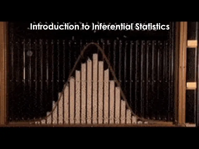
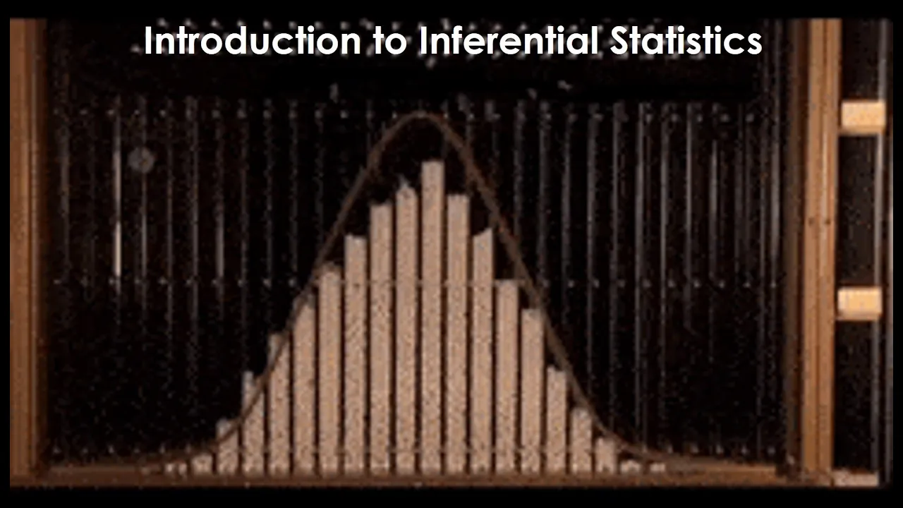
Hello and welcome back to clinical research method! Today i'd like to introduce you to the inferential statistics. As you probably know many research rely on a single sample assuming that they're randomly drawn from the population with a handful number of patients, subjects, participants, cell lines, and so on but if we think about it why do people conduct their research with the sample?
It is not like they are interested in the specific individuals in the sample, are they? Unless you are interested in very rare cases or phenomena on their own, the reason for studying a sample in general is not to learn about individuals in the sample but rather to infer certain population characteristics that the sample represents. So depending upon what you want to do with statistics, the goal of statistical analysis can be either a descriptive or inferential where descriptive statistics is mainly about describing the sample characteristics by summarising and visualising to better understand the data collected and measured from a sample which is what we have done so far in the exploratory data analysis.
On the other hand, the goal of the inferential statistics is to make an inference about the population of which characteristic is represented by the sample and understandably one of the practical reasons why we study a sample is that the population is typically too big to study and we only have limited resources in terms of time and money. Typically the size of a sample is only a tiny fraction of a population and the question of inference then is about quantifying our degree of confidence on how representative the sample is of the population. So let's consider Scottish population which is currently about 5.
5 million people. So here the big n represents the number of population, not normal distribution, and here say we take a sample from the Scottish population and here the small n represents the size of the sample so let's say that the population characteristic of potential research interest for vision scientists may be the intraocular pressure of the population and you want to have a single number that is representative of or typical of Scottish population so as we learned previously on average or the mean can be one of the summary statistics we can use but to calculate the mean for the population then we need to know every single intraocular pressure of all the members of population and obviously it is not feasible to measure and record the whole five and a half million IOPs so instead what's done in practice is that we collect a small fraction of the population and then measure the IOP of the sample and estimate the population IOPs from the average sample IOP. So for example, let's say you have this sample of Scottish population with the size of 27 so you can see that this is a much doable now and to measure 27 IOPs instead of some you know five and a half million IOPs now we can calculate the mean of the sample which turned out to be 17.
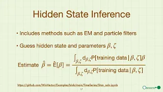
5 millimeter mercury then another question is how much confidence do we have about the unknown population mean intraocular pressure based on the sample statistics we have at hand. So that is the question of the inferential statistics how do we estimate the population characteristics from the given sample and quantify our uncertainty or certainty about the estimate we have at hand. So here the statistics is a characteristic of a sample and x bar as we have learned previously represents sample mean and the goal of the inferential statistics is to estimate the population parameter mu so population parameters the parameter is the characteristic of the population whereas statistics is the characteristic of the sample now then the goal of the inferential statistics is to say something about the population parameter from the sample and the parameter is typically denoted by these greek letters so mu represents the population mean the population mean when x bar is a sample mean.
So here are the words that we used in the previous slides so here I'd like to have a brief definition of each of them so the population is a collection of all subjects, samples, or participants of interest. So in our example our population was the people living in Scotland so that is the people living in Scotland and the parameter is a summary characteristic of the population in our case it was the mean population IOP of the people living in Scotland and then from this population we have a sample right which is a subset of the population of interest so for example say students from the clinical research method class can be a subset of the population of interest even though it is not a random sample technically speaking but the statistics is a summary characteristic of the sample right so in this case it is going to be the sample mean of intraocular pressure of the clinical research method class and the subjects of this story is the units of sample on which characteristics are measured so individual students will be an example of the subject in our case and then finally the variable that we are measuring which is the characteristic which are being measured and or recorded and in our cases intraocular pressure. So let's go back to the problem of estimating the population intraocular pressure from a sample so if you think about it studying a sample mean seems kind of meaningless to find about the population average because every time we take a sample here we assume the sample is drawn at random the sample mean IOP that the average IOP of the sample will change because the members of sample will change as you can see from here.
So then you know what can we say about the population parameter from a sample statistics? Intuitively we can say that we will have a better estimate of the population mean if we increase the sample size and then sample mean will approach to the population mean and it will become the population mean when the sample size becomes the size of the population so long time ago some genius mathematicians thought about this relationship between the sample size and the accuracy or the precision of a parameter estimation. So they thought "Is there any lawful behavior of sample mean given the size of the sample in relation to the true population mean from which the sample is drawn randomly to show how close or far away the sample mean is to or from the true population mean unknown to us?
" So when a large number of sample means with the same size are and randomly drawn from a population then the resulting distribution which is known as sampling distribution of the means show the interesting mathematical properties that have enabled us to create numerical methods that measure how much we should be confident that the sample represents the population we are studying. So for the sake of illustration let's pretend that we somehow know how the population distribution look like which is represented by the red curve here so the population intraocular pressure are normally distributed with a mean of 17 millimeter mercury and a standard deviation of 6 millimeter mercury. So now imagine that we draw a thousand samples of size four from this population with replacement, meaning that after a member is selected at random from the population then it is returned to the population and then the next member is selected at random so with replacement sampling there is still a chance for the first drawn member to be picked again.
So having said that, now each time we select four members then we finish collecting a sample in this kind of simulation. So for example then we measure each member's intraocular pressure and calculate the sample mean so for example here is our first sample mean of 17. 5 millimeter mercury.
Done. so next we put all these four members back to the population and draw another sample of four and measure the individual IOP and calculate the sample mean for the sample and this time the mean is 17 millimeter mercury so you repeat this procedure until you have a thousandth sample of four which now has a sample mean of 18. So of course each sample mean will be different from each other because every sample is composed of different members of population so now you have collected thousand sample means and we can construct a histogram of these sample means.
So this is the result of what is called the sampling distribution of the mean which is depicted by the grey histogram in the middle so remember our population was known to us already and then is represented by the red curve here right and the gray histogram is the histogram of the 1000 sample means of size 4. So if we look at the histogram it looks more or less normally distributed with its centre is on top of the population mean of 17. So this black line represents the mean or the centre of the sampling distribution of the mean which is this one so that's this histogram right so that looks like a normally distributed and the centre of this histogram is actually right on top of the population mean of 17.
So this centre of the histogram represents the mean of the sample means not the mean of a sample This is different from your usual histogram and another feature of the histogram is the smaller spread compared to the population distribution right so that is where the standard deviation of the sampling distribution and this red one this is the standard deviation of the population and it turns out the standard deviation of the sampling distribution of mean is actually smaller than the population standard deviation by the square root of the sample size as is depicted here right so the 6 and the numerator was the original population standard deviation and if we divide the standard deviation by square root of the sample size so square root of four is two so six over two becomes three so the standard deviation of the sampling distribution is 3 right that's 3. So is it? You're not sure about this so you decided to change the sample size to nine to see what happens.
So we repeat the same process take a sample of size nine now and measure the sample mean IOP. put them back to the population and pick another sample of nine measure the sample mean IOP so you do this another 998 times to collect thousand sample mean IOPs and construct a histogram of those thousand sample means and see what happens and voila! Now the blue histogram is the distribution of the sample mean of size nine again the mean of the sampling distribution is again on top of the population mean of 17 but the standard deviation got smaller than before by how much?
by the square root of the sample size of nine! see here so the square root of nine is three so six over three is two so let's just do this one more with a different sample size at this time we're going to increase the sample size to 36. and as expected the mean of the yellow histogram is the same as the population mean with the smaller even further smaller standard deviation than the population standard deviation by the square root of sample size of 36.
So square root of 36 is six so six over six is one so as you can see if we increase the sample size to the infinity then the standard deviation of the histogram will approach to zero and the sample mean will become exactly the same as the population mean. In a nutshell, this is basically what came to be known as the central limit theorem so here is kind of a formal description of the central limit theorem by Laplace who actually rediscovered the central limit theorem. So he's not the first one who actually theorise it.
That was de Moivre of and who was the predecessor of Laplace but he actually rediscovered it and then and organised it in one of his publications. So what the central limit theorem is a bit mouthful but I'll just read it verbatim. So when sample means each consisting of a sample size n randomly selected from a population are obtained from an unlimited series of random sampling with replacement and the resulting distribution of the sample means, also known as sampling distribution of the mean, will be approximately normal, normal as in normal distribution regardless of the shape of the population distribution from which the samples are drawn as the sample size n increases.
So according to the central limit theorem, a sampling distribution of the means displays the following behaviours. So the mean of the sampling distribution please note that this is not the individual sample means will be the same as the population mean so here the mu represents the mean of the sample means okay so here the data are sample means, not individual values okay and so if you have large enough sample size then it'll approach to the population mean right so the mean of the sampling distribution will be the same as the population mean so that's one of the properties of the sampling distribution and the other behavior of sampling distribution is that the standard deviation so here sigma represents the standard deviation of the sample mean x bar equals to the population standard deviation so this is the population standard deviation and divided by the square root of n which is the sample size and this standard deviation of a sampling distribution of means also known as standard error of the mean so standard of the mean so standard error of the sample mean is denoted as s. e.
m. or s. e.
for short and this is basically the standard deviation of the sampling distribution and the size of the standard error will give you a measure of how precise your estimation of that population mean so if you think about it, the standard deviation of a sample will provide how close the data in the sample are to the sample mean on average. However to say something about the population mean from the sample mean we need to know how close the sample mean is to the population mean and the standard error of the mean will provide us with that information so the sample means will vary less from sample to sample by the square root of the sample size according to the central limit theorem so what that means is that if you have a large sample size then your estimation of the population mean will become more and more precise okay but on the other hand a large standard error of the mean sem means that your sample might not be very representative of the population. Another property of the sampling distribution is its robust normality.
So intuitively if the sample generating population is normally distributed then you would think that the resulting sampling distribution will be normally distributed too however even if the population is not normally distributed sampling distribution will be more or less normally distributed with a reasonably large sample size so here we say reasonably large so we're talking about larger than 30 or more sample size that's what we're talking about as a kind of a ballpark number so here we have a simulation of the property and where the top pinkish distribution is the original population from which sample means will be generated so obviously it is not normally distributed as you can see but rather it looks more like an exponential distribution so imagine that we simulate a central limit theorem using this population to see how the shape of the distribution sampling distribution changes as a function of sample size so on the left is showing a sampling distribution constructed from thousands of sample means with the size of 5 drawn from that top distribution and as is obvious, the shape of the sampling distribution does not look very normal but positively skewed or the skew to the right but as we increase the sample size to 30 and the resulting sampling distribution in the middle looks more or less normal with a slight positive skew and finally as the sample size increased to 100 and the sampling distribution on the right looks almost normal. So if our sample size is large enough say over 30 then we can assume that the sampling distribution, not the individual samples, will be approximately normal and what and what that means is that all the properties of normal distribution will apply to this sampling distribution. So for example we know that the true population mean will be located somewhere within plus minus 2 standard error of the mean of the sampling distribution which is.
. . so the two standard error of the mean is basically the standard deviation of the sampling distribution given the sample mean and the size.
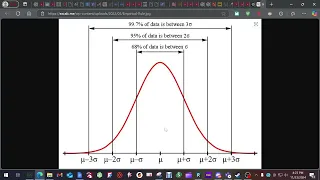
So when the sample means, not the sample data follow normal distribution with a population mean of mu and the standard error of the mean then it can be standardised using the z transformation as we learned before because the standard error of the mean is the standard deviation of the sampling distribution and then all the properties of normal distribution are applied to this distribution too such as 95% of the sample means will fall around the population mean so here you have just to be careful about this one so x bar when x bar follows the normal distribution with the mean of the population mean and then this sigma over square root of n is the standard deviation of sampling distribution so this is the standard deviation of the sampling means distribution of the sampling means which is known as standard error of the mean so that's s. e. m.
and we can standardise by subtracting the sample means, which is our data now from the population mean and divide this by the standard deviation of the sampling distribution of the mean which is the standard error of the mean right then it will so we can find so this is a plus minus one standard error of the mean and you will find 68 percent in the middle and within plus minus 2 standard deviation that you can find the 95 percent okay so that will become 95 percent 95 and so on and within plus minus three standard error of the mean you will find 99. 7 percent and especially this interval within plus minus two standard error of the mean is known as 95 percent confidence interval so here the CI stands for confidence interval um so this was first suggested by a statistician named Jersey Neyman in 1937 to report as a metric indicating how accurate our estimate of the population mean will be given the sample mean and the size so the confidence interval is an observed boundary from the sample within which the unobserved parameter so in this case population mean would fall within a given confidence level and in practice we report our sample mean as our estimation of the population mean along with the confidence interval to express the amount of certainty or uncertainty in the estimation and you can use different levels of confidence but 95 is the most commonly used confidence level. So in practice, it is quite a standard procedure to report 95 confidence interval along with the sample mean and it is not that difficult to calculate as you can see from the simple equation so the lower boundary of the any percent level there's a given level of confidence the lower boundary of the confidence interval is x bar which is the sample mean that you measured minus the z this is kind of the confidence level you're going to use and most commonly used confidence level is 95 right which correspond to the set score of 1.
96 or rounded up to two and you multiply this by standard error of the mean which is basically the standard deviation of the sample and then square root of n so that's so because you don't know the population standard deviation right you use the sample standard deviation instead as if this is the population mean i mean population standard deviation sorry and then you divide this by the square root of the sample size that of your sample right so that is the lower boundary and the upper boundary is just to add this amount to the sample mean then you will have the upper boundary of the confidence interval so for the 95 confidence interval it is basically sample mean plus minus 2 standard error of the mean. So that's all there is to it and given the same level of confidence interval say you have two sample means and then you calculate the 95 confidence interval for both sample means and if you have a wider confidence interval, that indicates your sample mean is less representative of the population mean. On the other hand, if you have narrower confidence interval right then that means your estimation of the population mean from the sample mean is quite accurate okay so this is almost like a rhetorical problem but if you have a large confidence interval, that means you're not very confident if you have a small confidence level then that means you are confident about your estimation.
and also given the same sample mean, if you increase the the confidence level say from 95 to 99 then obviously your confidence interval gets larger, wider given the same sample mean because you become more conservative about your estimation by increasing the level of confidence. and it is also common to report plus minus one standard deviation instead of a 95 percent confidence interval along with the sample mean but if you do that then it has actually slightly different meaning compared to the confidence interval so they serve different purposes and that many people are not very attentive to so if you want to indicate the average variability of the data or observations in the sample then you will use standard deviation. On the other hand if you want to indicate the uncertainty the amount of uncertainty you have in the estimation of the unknown population mean then you will report the confidence interval.
So let's calculate the 95 confidence interval using an example. Let's say that you measured the intraocular pressure of a sample the size of with the size of 36 patients and you calculate the average intraocular pressure for this sample and also standard deviation so when you have a sample like this can calculate the 95 confidence interval by calculating the the lower and the upper limits or the boundaries so let's just start with lower boundary first so that's x bar minus z star times standard deviation so I'll just say s over square root of n right so you just have to plug in and the number you obtained from your sample so x bar here is 17 minus because we're calculating the 95 percent confidence level the z star will be 1. 96 but you know for the sake of easier calculation I'll just use two okay and the standard deviation is 3 over 36 right so that becomes 17 minus and what's inside the bracket so square root of 36 is 6.
so that's 2 and cancel each other out so we are left with one so lower boundary is 16 so then upper boundary is basically the same but you just add the amount in the bracket. So that becomes 17 plus 1 and that is 18 right so that is the quantity from the bracket and it doesn't change right so we can just add this amount without having to calculate it again right so that's the lower boundary and upper boundary of this sample mean right so sample mean is 17 so x bar is 17 with 95 percent CI and you use square bracket to report and 16 and 18. lower boundary and upper boundary see so this is interval and you know that the sample mean should be located inside this 95 confidence interval and because we're assuming the normal distribution and the boundary should be symmetrical around the sample mean if it is not then there's something wrong and also if you don't see the sample mean inside this within this interval 95 confidence interval then also there's something wrong with the calculation so you can double-check if your calculation of 95 confidence intervals correct or not by placing the sample mean within the confidence interval you calculated so let's just then draw on an error bar using this 95 confidence interval so once you have the 95 confidence interval and and sometimes especially when you have kind of a two or more groups to compare then the error bar representation of your data is a very good visualisation because it gives you a quick information about the difference between these groups anyhow we're going to just talk more about this error bar visualisation later on when we're talking about the t-test but it is very easy to create an error bar so here on the y-axis we have the integral pressure right and you draw a bar so erect the bar corresponding to the sample mean here right so that is 17 milimetre mercury and then so from this bar you add add a line above and below the sample mean of which length corresponds to two standard error of the mean right it is plus minus two standard error the mean that is the ninety-five percent confidence interval CI so that's basically what it is ninety-five percent confidence interval and sometimes you can see that there is you know stopping bars like the horizontal stopping bar but this is optional you don't have to have that and even you don't even have to have this the bar around it you can just omit this right because you know that the mean is exactly in the middle of the 95 confidence interval sometimes people don't include this bar they only add error bar because that actually conveys enough information about the sample mean so this upper boundary is 18 right that's what we calculated before and then the lower boundary is 16 there right so this is how to create an error bar and then now we're gonna go to the summary.