The first documented negative feedback control system is generally believed to be the float regulator developed by Ctesibius in 270 BC. To maintain the water level in a tank, a wedge-shaped float would allow more water in when the level was too low and less water when the level was too high. Ctesibius created this without the use of a mathematical model of the system.
And it's not that Ctesibius chose to not use a mathematical model of the system. It's just that the mathematics hadn't been invented yet. And so he had to rely on trial and error and intuition to find the right equilibrium.
Fast-forward to the 1600s AD, during the Enlightenment period, where Newton and Leibniz were independently developing calculus and, from that, differential equations. A differential equation is an equation that relates one or more unknown functions and their derivatives. And this is important because this is one way that dynamic systems are represented mathematically.
If we call x the state of the system and u the external inputs into the system, then this is saying that how the system state changes over time is a function of the current state and external inputs. And with this framework, it was off to the races, creating mathematical models of dynamic systems. The likes of Euler and Lagrange and Maxwell and many, many others created mathematical models of the motion and behavior of solid mass, fluids, and of electromagnetic waves.
And this explosion of models led us to a much deeper understanding of the world and opened the door to using mathematical representation to design and test a system, rather than the trial and error of developing on the real system itself. Modeling is, of course, one of the six core capabilities crucial to a mature, model-based design development environment. And so it might come as no surprise to you that regardless of the industry you're working in, you'll probably find some form of modeling dynamic systems.
And so with that being said, I'd like to walk you through the map of modeling dynamic systems, which highlights many of the different tools and techniques that we have within MATLAB and Simulink. I think this is going to be pretty interesting. So I hope you stick around for it.
I'm Brian. And welcome to a MATLAB Tech Talk. The point of creating a model is so that you have a mathematical representation of your real system, whether that system is like a pendulum, whose model might be written directly as an ordinary differential equation, or a hybrid system with interacting continuous and discrete dynamics, or something like a walking robot, whose dynamics might be learned and captured with a neural network.
In each of these cases, we can split the model up into two different parts. There are the model parameters, or the variables, which we can think of as specific numbers within the model. And then there is the structure, which is the set of equations that establish the relationship between those variables.
So when we're creating a mathematical model of something, we have to think about which model structure we're going to use. And we have to think about how we find the model parameters that make up that structure. So how do we do that?
Well, this brings us to another thing we need to consider. And that is, where do you get the knowledge about your system so that you know which structure to use and you know how to get the parameters for that structure? If you understand the physical laws that govern your system, then you can derive the mathematical equations directly.
And this might mean using your knowledge of first principles and your knowledge of the system to write out a differential equation. Now, sometimes your system is too complex to easily write out a single set of equations. Or the equations aren't simple enough to be easily interpreted as to what they represent.
So in those cases, you can also build up a model with smaller mathematical components that are then connected together graphically, like you do in Simulink. And even without knowing how to create and manipulate differential equations, you can also create a model with a physical modeling system like Simscape. And this is where you connect physical components together, like mechanical, hydraulic, and electrical components.
And then the software takes care of the differential equations under the hood. So, for example, a mass-spring-damper could be modeled with the Simulink blocks on the left or, equivalently, as a physical model with the Simscape blocks on the right. And this type of physical modeling is really helpful when you start dealing with multibody dynamics.
You can see how much more complex the differential equations become for a double mass-spring-damper system compared to the equivalent physical component model. But in both of these cases, we're using our knowledge of the physical laws of the system to develop a model. We have to know that we're modeling mass-spring-dampers and how many there are and what their parameters are in order to develop these models.
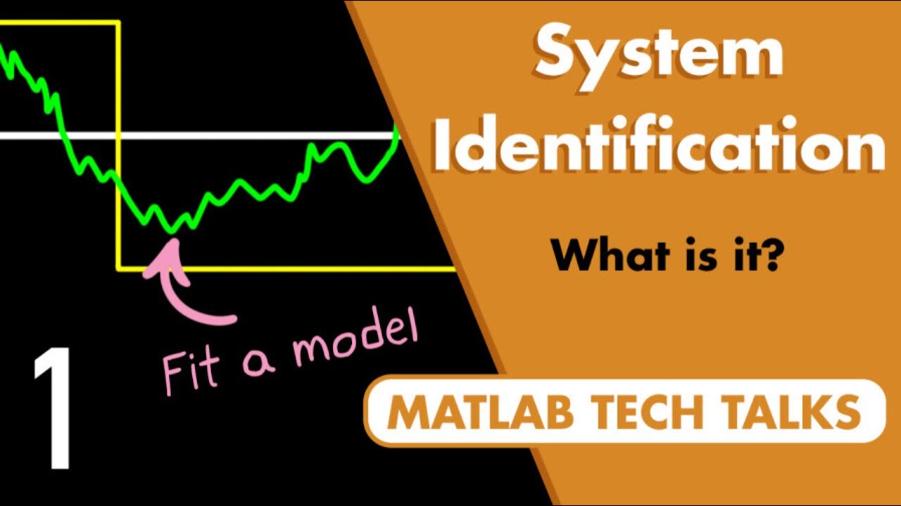
And this type of modeling is often referred to as the white box method. And on the opposite end of this is the black box method, where you don't necessarily know the physics of your system. But what you do have is data from the system.
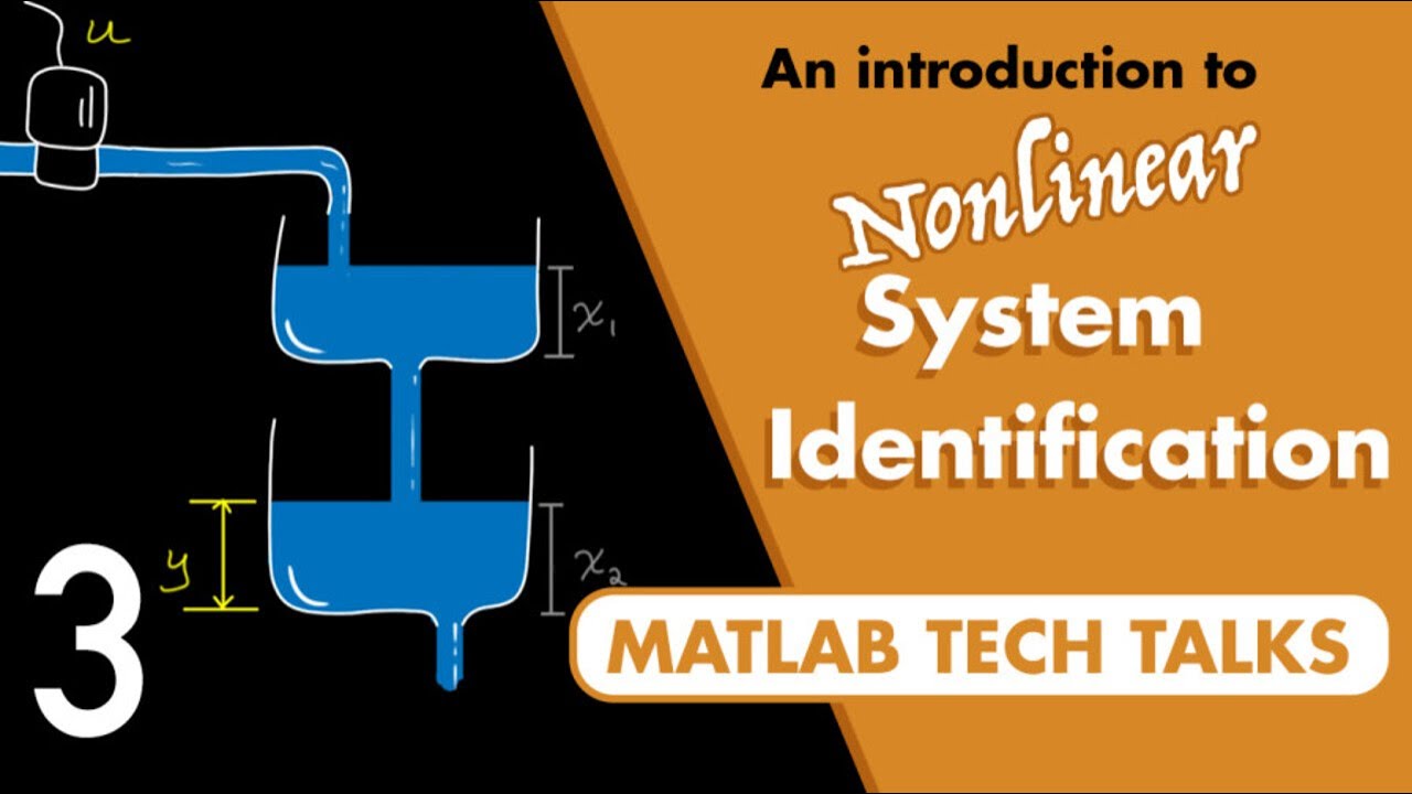
In this case, you can use that data to fit a model using a process called system identification. And there are many different methods for system identification. But regardless of the method used, the bottom line is that you're using data to understand the relationship between the inputs into the system and the outputs that it generates.
So even if you aren't left with a model that reflects the physics of the system, you still have something that captures the behavior of the system. And part of the system identification process is to prepare the data. And these are things like removing outliers and dealing with missing data points and such.
Then estimating the model can be done online, where the model is updated as new data is available, or offline, where the model is fit to a set of prerecorded data. And finally, the model needs to be analyzed. How good of a fit is it to the training data?
And how well does that model match test data? Model analysis also allows you to figure out the best order and structure of the model that you're fitting. And MATLAB has the System Identification app that will help you through this process.
Now, in between the black box and the white box methods is what we call gray box modeling, which is where you use some physical knowledge of the system to create the model. And then you learn the rest with data. For example, if you're trying to model an electric motor, you might choose an ordinary differential equation for a generic motor and then use data to learn the specific parameters for your motor.
And using data to estimate parameters is not just limited to MATLAB models but can also be done with Simulink models. In this way, you can build a model based on what you know and then learn the rest using data from the system. And there's the Parameter Estimator app, which can help with this type of gray box modeling.
Now, estimating model parameters is just half of the modeling story. Like we said, the other half is choosing a model structure. In what mathematical format do you want to capture the dynamics of your system?
Now, not only does the model structure need to be able to capture the dynamics, but it also has to be a structure that is right for the scenario under which you're going to use the model. For example, if you're looking for the ability to assess stability and performance and easily manipulate the system for design changes, then you almost certainly can't beat the simplicity of linear models. Of course, that's assuming that your system behaves linearly enough around an operating point that these models make sense.
Popular linear model structures are things like transfer functions and zero-pole-gain models, which are in the S and Z domains, and then state space and ARX and ARMA models in the time domain. And if you have frequency information from your system, from something like a sine sweep, then a frequency response data model might be a good choice. And a linear parameter varying model can be used if your system dynamics vary in a way that can be captured with time-varying parameters called scheduling parameters.
Now, for systems that are so nonlinear that a linear model doesn't suffice, you can move up to nonlinear model structure. And these are structures like ordinary differential equations, where you can capture the nonlinearities with an interpretable mathematical equation. Or you can use a deep neural network to represent the state space equations.
These are the state equations where x dot is some function of state x and input u and the output equations where the output y is a function of x and u. There are also some structures like Hammerstein-Wiener and nonlinear ARX that combine linear models with nonlinear components. And these are useful because they provide the best of both worlds, where you model the linear components of your system with simpler equations and then capture the nonlinear portion separately.
And the nonlinearity could be represented with a number of different structures, like polynomials and dead zones and piecewise linear. But you can also capture the nonlinearity with AI-based structures, such as Gaussian processes, support vector machines, regression trees, and neural networks. You can also integrate third-party models into MATLAB and Simulink.
So if you already have a model in, say, for example, Python or in C or some other supported tool or language, then you can pull those models into MATLAB and Simulink using functional mock-up units, Python importers, and S functions. All right. So now we've created a model.
We've picked a structure. And we've defined the model parameters through first principles, gray box, or data-driven methods. But you'll often find that a model might not be in the right format for what you want to use it for.
You may need to manipulate it or change it in some way so that it becomes useful for a different purpose. For example, you might need to transform the model to a different type, going from a transfer function to a state space model. Or you may need to change the domains that it's operating in-- so to go between continuous and discrete domains.
You may also need to manipulate a state matrix, where you can do things like switch between having the eigenvalues along the diagonal so that you have a sense of which modes exist in the system versus a format where the system states are possibly more aligned with the physical attributes of your system. Or you may want to decompose a larger model into smaller models that make it up. And all of these things fall under the umbrella term of model transformation.
Similarly, you may also start with a nonlinear model and then want to create a linear version of it through linearization. Nonlinear models are great for simulation because they tend to more accurately represent reality. But they may be harder to analyze and harder to design around.
And so you may want a linear equivalent of your nonlinear model at some operating point. And this can be done through numerical perturbation, where you start at the operating point, and then you perturb the parameters in both directions to find the slope. Linearization can also be done block by block, where you specify the Jacobian for each block within your Simulink model.
You can linearize also with frequency response estimation, where you excite your system at specific frequencies and then measure the response in terms of gain and phase shift. And like we've seen before, there's an app for this. The Model Linearizer app can help you through the entire linearization process.
And finally, you may have a high-fidelity model that accurately captures the hardware behavior. But it might not be suitable for different stages of the development cycle, such as for "hardware in the loop" testing or for system analysis and simulation. And so you may want to reduce a model down to something more manageable while maintaining the key dynamic characteristics.
And you can do that through model-based applications like balanced truncation and pole-zero simplification, both of which are available within the Model Reducer app. Or you may want to take a more data-driven approach, where you use data from your high-order model to learn or identify a lower order model, just like you would do with system identification. And the Reduced Order Modeler app makes this process really easy.
All right. So that's an overview of the map of modeling dynamic systems. And I think the key takeaways here are that it's good to have options and tools for creating models because there isn't one perfect approach.
It depends on the system that you're trying to model and the knowledge and data that you have about that system. Plus, it's important to know that modeling complex systems could use a combination of these tools. And if you want to learn more about anything that's on this map, as well as many other things that have to do with modeling dynamic systems, we've put together a page on mathworks.
com that gives you more information on each of these topics. There's a link to it down below, but also, the QR code at the top of the map will take you here as well. And it's got tons of great information.
So I hope you check it out. All right. That's where I'm going to leave this video.
I hope this map is at least a little bit useful when trying to navigate the world of modeling dynamic systems. Thanks for watching.