The field of software analysis is highly diverse. There are many approaches with different strengths and limitations in aspects such as soundness completeness Applicability and scalability. In this lesson we will introduce Dataflow analysis one of the dominant approaches to software analysis.
We will see specific examples of useful dataflow analysis from the literature. And we will learn about a general technique to design a dataflow analysis. After this lesson you should be able to design your own dataflow analysis for a basic yet powerful programming language that captures the essence of realistic programming languages like C and Java.
Dataflow analysis is a kind of static analysis for reasoning about the flow of data in runs of a program. The data can be of different kinds: constants, such as the number 7 or the string literal "hello", variables such as foo, expressions such as 7*foo, and so on. This information in turn is used by bug finding tools to find programming errors and by compilers to generate efficient code for the given program.
Throughout this lesson we will work with a simple programming language called the WHILE language. Here is an example program written in this language to compute the factorial of 5. The program has two integer variables x and y.
It initializes these two variables and then updates them in a loop. Variable x contains the factorial of 5 at the end of the program. Here is a formal grammar that precisely describes the syntax of programs written in the WHILE language.
You can learn more about this notation by clicking on the link in the instructor notes. A program in this language is a statement S, which can be an assignment statement, a sequential composition of two statements , an If-Then-else statement, or a while statement. Notice that this definition of a statement is recursive, so it can be used to describe arbitrarily large programs.
Programs with nested if/then/else statements, programs with nested loops, and so on. For simplicity we have only integer variables in this language. Furthermore assignments to such variables can only be arithmetic expressions of a limited form.
In particular an arithmetic expression can be an integer variable, which we denote using x or an integer constant which we denote using n, or a multiplication of two expressions, or a subtraction of one expression from another expression. Notice that the definition of arithmetic expressions is also recursive, allowing us to write programs with arbitrarily large expressions. It's easy to extend the syntax of these expressions to include other operators such as addition and division.
But we will leave those out for now to keep it simple. Finally to express conditions in If-then-else statements and while statements we have boolean expressions. A boolean expression may be the constant true, the negation of another boolean expression, the conjunction of two boolean expressions b1 and b2, or a comparison between two arithmetic expressions a1 and a2.
Again to keep things simple we allow limited kinds of Boolean expressions. Although it is easy to extend the syntax of this language to include operators besides the ones shown here. Notice that the WHILE language does not have any fancy constructs such as functions, pointers or threads, that are provided in commonly used programming languages such as C and Java.
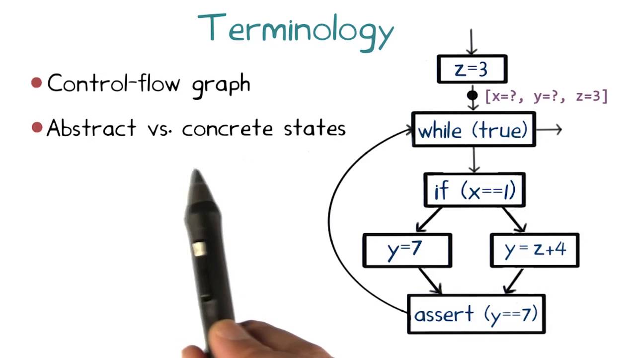
This is because the presence of loops already makes the while language expressive enough that interesting properties of programs written in this language are undecidable and yet simple enough to allow us to study the fundamentals of dataflow analysis. Dataflow analysis typically operates on a suitable intermediate representation of the program. One such representation shown here which we also saw earlier in this course, is a control-flow graph a control-flow graph is a graph that summarizes the flow of control in all possible runs of the program.
Each node in the graph corresponds to a unique primitive statement in the program, such as an assignment, or a condition test. And each edge outgoing from a node denotes a possible immediate successor of that statement in some run of the program. Take a moment to convince yourself that this graph is indeed a control-flow graph of this program.
To check your understanding of control-flow graphs let's do an exercise converting a control-flow graph into the program it came from. Here is a control-flow graph. In the adjoining box write the program corresponding to this control-flow graph in the syntax of the WHILE language.
Click the submit button to check your answer. Recall from before that it is impossible to design a software analysis that is sound, complete, and guaranteed to terminate. This impossibility holds for dataflow analysis as they too are a kind of software analysis.
Dataflow analysis choose to sacrifice completeness but guarantee termination and soundness. Since dataflow analysis is sound it will report all dataflow facts that could occur in actual runs of the program. However, because dataflow analysis is incomplete it may report dataflow facts that can never occur in actual runs.
Let's see next how a dataflow analysis achieves soundness by sacrificing completeness. The primary source of incompleteness in dataflow analysis arises from abstracting away control-flow conditions with non-deterministic choice. Which we will denote throughout this course using the * symbol.
For this example program dataflow analysis replaces the condition x! =1 with non-deterministic choice. Non-deterministic choice simply means that the analysis will assume that the condition can evaluate to true or false.
Even if, for example, in actual runs the condition always evaluates to true. By doing this, not only does a dataflow analysis ensure that it will consider all paths that are possible in actual runs of the program, and thereby guarantee soundness, but it also considers paths that are never possible in a actual runs which leads to incompleteness. We will learn how dataflow analysis works on a control-flow graph through a series of four classical dataflow analysis in the literature.
These analyses are: reaching definitions analysis, very busy expressions analysis, available expressions analysis, and live variables analysis. Before we dive into the details of these four analyses let's take a look at four practical applications that motivate them. Reaching definitions analysis produces information that can be used by a software quality tool for discovering uses of potentially uninitialized variables in a program.
Very busy expressions analysis computes information that can help reduce code size. This application can be critical to certain embedded devices that have code size constraints such as pacemakers. Available expressions analysis produces information that can be used by a compiler to avoid recomputing the same program expression multiple times in an execution.
Thereby producing more efficient code. And finally, live variables analysis computes information that can be used by a compiler to efficiently allocate registers to program variables. Register allocation is the component of a compiler that most impacts the performance of the generated code.
Next we will dive deep into how each of these four analyses work starting with reaching definitions analysis. We will use reaching definitions analysis to introduce the key concepts of dataflow analysis. Each dataflow analysis has a goal that specifies the kind of dataflow information that the analysis computes.
The goal of reaching definitions analysis is to determine which assignments might reach each program point. More accurately this analysis determines for each program point which assignments potentially have been made and not overwritten when the program's execution reaches that point along some path. For the purpose of this analysis, we will use the terms assignment and definition interchangeably.
Since an assignment corresponds to a definition in the WHILE language let us look at the following example program. There are four definitions in this program: x is assigned y y is assigned 1, y is assigned x * y, and x is assigned x-1. Consider two program points P1 at the Entry of this condition, and P2 at the exit of this assignment.
Let's consider the definition x is assigned y. This definition reaches the program point P1 as there is no overwriting assignment to x along this path. But this definition does not reach the program point P2 as x is overwritten by the assignment x is assigned x-1 every time execution reaches P2.
Please take a moment to understand the goal of reaching definitions analysis. We will next do a quiz to practice a few more reaching definitions in this control-flow graph. To check your understanding of reaching definitions analysis here's a short quiz.
Check the boxes corresponding to the statements that are true about reaching definitions analysis. Informally speaking the result of a dataflow analysis is simply a set of facts at each program point. For example, reaching definitions analysis computes the set of definitions that may reach each program point.
We will denote each such definition as a pair comprising the name of the defined variable along with the label of the node that defines it. For example the definition of variable x at the node label 2 is denoted as follows, and the definition of variable y at the node labeled 5 is denoted as follows. Now let's make the notions of a program point and dataflow analysis result more precise.
To identify each program point uniquely let's assign a distinct label to each node in the control-flow graph. I have labeled the nodes in this control-flow graph from 1 through 7. Then, for each node with Label n we use IN of n to denote the set of facts at the entry of node n, and OUT of n to denote the set of facts at the exit of the node.
A dataflow analysis computes the IN and OUT sets of facts for each node in the control-graph. It does so by repeatedly applying two operations until the sets of IN-and-OUT facts for each node in the graph stop changing. At that point, we say that the result of the dataflow analysis is saturated, or that it has reached a fixed point.
We will next introduce these two operations for reaching definitions analysis. Subsequently, we will see slight variations of these operations for the other three dataflow analysis. Here is the first of the two operations of reaching definitions analysis.
This operation states how to compute the set of facts at the entry of a particular node in the control-flow graph. We do this by taking the union of the sets of facts at the exit of that node's immediate predecessors. That is, the union of OUT(n') for each predecessor node n' of n.
The second operation of reaching definitions analysis tells us how to compute the set of facts at the exit of a particular node from the set of facts at the entry of that node. Unlike the previous operation that we just saw, this operation depends on the statement that occurs at the node we are looking at. We will first state this operation in its general form and then we'll show specific instances of it corresponding to each kind of primitive statement in the WHILE language.
The general form of this operation states that the set of facts at the exit of node n is equal to the set of facts at the entry of node n minus any definitions that are overwritten by node n union with any definitions that are generated by node n. We call these sets of definitions the KILL set and the GEN set respectively. Determining the GEN and KILL sets requires knowledge of the statement that occurs at node n.
For control-flow graphs of programs in the WHILE language this statement can be either a condition or an assignment. Let's consider each of these two cases in turn. If the statement at node n is a condition then both the GEN and KILL sets are empty.
Since there are no definitions overwritten or generated by a conditional statement. So in this case the set OUT(n) will be equal to the set IN(n). If the statement at node n is an assignment of the form x is assigned a, then the GEN and KILL sets are more interesting.
The GEN set contains the definition of variable x at node n itself, reflecting the fact that this definition is generated by node n. The KILL set, on the other hand, contains every definition of variable x except the one at node n, reflecting the fact that all those definitions will be overwritten by the one at node n. We denote this set compactly using set comprehension notation.
You can review this notation by following the link in the instructor notes. Equipped with the two operations of reaching definitions analysis, let's step through the overall reaching definitions analysis algorithm. The algorithm starts by initializing the IN and OUT set of each node n in the control-flow graph to the empty set.
The only exception is the OUT set of the entry node of the control-flow graph which is initialized to contain a hypothetical definition for each variable v in the program. It captures the fact that each variable is undefined or uninitialized at the start of the program. The algorithm then performs its main task from which it derives the name Chaotic Iteration Algorithm.
The name highlights two important properties of the algorithm. First, it is iterative. It repeatedly updates the IN and OUT sets of each node in the control-flow graph until they stop changing.
Second it is chaotic in the sense that in each iteration it visits all the nodes in the control-flow graph and applies the two operations we just discussed to update the IN and OUT sets of each node. Crucially the order in which the nodes are visited does not matter lending the adjective chaotic in the name of the algorithm. Now let's see how the chaotic iteration algorithm for reaching definitions analysis works on our example control-flow graph.
We will use this table to track the values of IN and OUT sets of each of the 7 nodes in this control-flow graph. The algorithm starts by initializing all these entries to the empty set, except for the OUT set of the entry node, which captures the fact that both variables x and y are undefined at this point. Also, we will ignore the IN set of the entry node, and the OUT set of the exit node, as these nodes do not contain any statement and are merely placeholders.
Next, the algorithm repeatedly picks each of the remaining 5 nodes and applies the two rules that update their IN and OUT sets. It also updates the OUT set of node 2 to reflect the fact that the definition of variable x generated at node 2 reaches the exit of node 2. Notice that node 2 also kills the incoming fact that x is undefined.
But it retains the incoming fact that y is undefined. Likewise it updates the IN set of node 3 to reflect the fact that the definition of x at node 2 reaches it, and the fact that y is still undefined. Continuing further, it updates the OUT set of node 3 to reflect the fact that not only is the incoming definition of variable x not overwritten by node 3, but furthermore node 3 generates a new definition of variable y.
Both these definitions reach the exit of node 3. Recall that the IN set at node 2 contains the hypothetical definition of variable y indicating that y is uninitialized at this point. A bug finding tool could use this information to deduce that the use of variable y at node 2 might be uninitialized which is a potential programming error.
Let's update the remaining entries of this table in the following quiz. Fill-in the blank entries in the table with the final values of the corresponding IN and OUT sets computed by the chaotic iteration algorithm for reaching definitions analysis. Keep in mind the two operations that the algorithm applies to each node.
The first operation states that the IN set of a node is the union of the OUT sets of its immediate predecessor nodes. The second operation states that the OUT set of a node contains all the definitions in the IN set of that node minus definitions that are overwritten by that node, plus any new definitions that are generated by that node. Remember to keep iterating through the whole table applying these two operations to each node until there are no changes in a given pass through the table.
At this point you might be wondering whether the chaotic iteration algorithm is guaranteed to terminate for every program in the WHILE language. Despite its seemingly chaotic nature, the answer perhaps somewhat surprisingly, is yes. The reason for this is twofold.
First the two operations that this algorithm applies in each iteration are monotonic. That is they never cause the IN and OUT sets to shrink. We indeed observe this behavior in the table of the reaching definitions example where these sets always grew bigger.
Secondly the largest that any such set can get is the set of all the definitions in the program which is finite. This implies that the IN and OUT sets cannot grow forever. Together these two reasons ensure that all IN and OUT sets will stop changing in some iteration of the chaotic iteration algorithm, which is the condition under which that algorithm terminates.
Now let's move on to the second of the four classical dataflow analysis. This one is called very busy expressions analysis. We will present this analysis by following a recipe similar to the one we used to present reaching definitions analysis.
The goal of very busy expressions analysis is to compute expressions that are very busy at the exit from each program point. An expression is very busy if, no matter what path is taken, the expression is always used before any of the variables occurring in it are redefined. Let us look at the following example program.
Let's consider these two expressions in this program: a-b and b-a. Consider this program point P at the entry of this condition statement. The expression b-a is very busy at this program point since it is used along both paths from that point.
Before any of the variables occurring in this expression is redefined. Now let's consider the expression a-b. This expression is used on both paths as well.
But notice that variable a is redefined along one of those paths before the expression is used. Hence expression a-b is not considered very busy at the program point P. Here is the first of the two operations of very busy expressions analysis.
This operation states how to compute the set of facts at the exit of a particular node in the control-flow graph. We do this by taking the intersection of the sets of expressions at the entry of that node's immediate successors. That is the intersection of IN of n' for each successor node n' of n.
The second operation of very busy expressions analysis tells us how to compute the set of facts at the entry of a particular node from the set of facts at the exit of that node. The operation of this rule depends on the statement that occurs at the node we are looking at. Like we did for reaching definitions analysis, will first state this operation in its general form and then we'll show specific instances of the operation corresponding to each kind of primitive statement in the WHILE language.
The general form of this operation states that the set of very busy expressions at the entry of node n is equal to the set of expressions at the exit of node n minus any expressions using variables that are modified by node n unioned with any new expressions that are used by node n. Like before, we call these sets of expressions the KILL set and the GEN set. If the statement at node n is a condition statement then the KILL set and the GEN set are empty since nothing is modified nor generated by this node.
If the statement at node n is an assignment statement of the form x is assigned a, then the GEN set will contain the expression assigned to variable x at node n itself, reflecting the fact that this expression is used by node n. The KILL set, on the other hand, contains every expression using x, reflecting the fact that all those expressions will be modified by node n. The overall algorithm for very busy expressions analysis is nearly identical to that for reaching definitions analysis.
But it has three notable differences. First, the two operations that are applied in each iteration of the algorithm are slightly different. Notice that the roles of the IN and OUT sets in these two operations are switched, reflecting the fact that very busy expressions analysis propagates information backwards in a control-flow graph, in contrast to reaching definitions analysis which propagates information forward.
Moreover, we take the intersection of sets as opposed to their union which causes the IN and OUT sets of very busy expressions to shrink as the algorithm progresses. In contrast, recall that in reaching definitions analysis the IN and OUT sets of reaching definitions grew because we used the union operation. This also makes it clear why we initialize all IN and OUT sets in very busy expressions analysis to the set of all expressions in the program since these sets will shrink as the algorithm progresses.
In contrast, recall that the IN and OUT sets in reaching definitions analysis were initialized to the empty set and those sets grew as the algorithm progressed. However, by convention, we will still set the IN set of the exit node of the control-flow graph to be empty since no expressions are very busy at the end of the program. Now let's see how the chaotic iteration algorithm for very busy expressions analysis works on our example control-flow graph.
We will use this table to track the values of the IN and OUT sets of each of the 8 nodes in this control-flow graph. The algorithm starts by initializing all these entries to the set of all expressions. Except the OUT set at the exit node, which it initializes to the empty set.
As in the case of reaching definitions analysis, we will ignore the IN set of the entry node and the OUT set of the exit node as these nodes do not contain any statement and a merely placeholders. The Algorithm repeatedly picks one of the remaining nodes and applies the two rules that update their IN-and-OUT sets. For instance, it updates the OUT set of node 7 to the empty set, reflecting the fact that no expressions are very busy at this point.
Likewise it updates the IN set of node 7 to reflect the fact that expression a-b is very busy at this point as it is indeed used immediately thereafter. Continuing along this branch it similarly updates the OUT set of node 6 to the empty set as no expressions are very busy at this point. Similarly it continues further back and updates the IN set of node 6 to reflect the fact that expression a-b is very busy at this point.
Let's update the remaining entries of this table in the following quiz. Fill-in the blank entries in the table with the final values of the corresponding IN and OUT sets computed by the chaotic iteration algorithm for very busy expressions analysis. Keep in mind the two operations that the algorithm applies to each node.
The first operation states that the OUT set of a node is the intersection of the IN sets of its immediate successor nodes. The second operation states that the IN set of a node contains all the expressions in the OUT set of that node minus expressions that are overwritten by that node plus any new expressions that are generated by that node. Remember to keep iterating through the whole table applying these two operations to each node until there are no changes in a given pass through the table.
Next let's move on to the third of the four classical dataflow analysis, called available expressions analysis. The goal of this analysis is to determine for each program point which expressions have already been computed and not later modified on all paths to the point. Let us look at the following example program.
There are three expressions of interest in this program a-b, a*b and a-1. Consider the program point P at the entry of this condition. At this point the expression a-b is set to be available.
To see why let's show that this expression is already computed and not later modified along every path that reaches this point. There are two paths. Along this path the expression a-b is computed here and neither a nor b is modified later.
Likewise, along this path, the expression a-b is computed here and neither a nor b is modified later. On the other hand, the expression a*b is not available at program point P. This is because although this expression is available along this program path, it is not available along this other program path.
In particular, the variable a occurring in this expression is modified here along this path. And moreover this expression is not computed after that modification in order to become available later at the program point P. Let's walk through an example.
Our IN set in this case will be any expressions which have been calculated earlier in the code without having the variables in their calculations overwritten. Our OUT set will be our IN set minus any expressions which have a variable that is overwritten by that statement, plus any expressions that are generated by that statement. Let's walk through the first three program points.
For the entry node we have the empty set as our OUT set. This OUT set will be copied over to the IN set of node 2. To compute the OUT set of node 2, we first copy the IN set of node 2, which is empty, and add expression a-b which is generated at node 2.
Node 3 takes in the expression a-b from node 2. In addition, node 3 generates another expression a*b. qhich we add to its OUT set.
Node 4 is a bit tricky. Our IN set at this point is the expressions a-b and a*b. Note that this is not the only path to this program point.
But we have not computed the OUT set of node 4's other predecessor yet. So we need to make at least another pass through the table before the algorithms stabilizes. Nothing is killed at node 4 and so we copy the IN set to the OUT set.
Nothing is generated at node 4 either. And so we do not add any further expressions. At node 5 we first copy the OUT set of node 4 to the IN set.
Node 5 seems to generate the expression a-1 but in fact it does not since it immediately overrides the variable a. Also, we'll need to kill each expression in our IN set that uses variable a. That's expressions a-b and a*b.
So, we are left with an empty OUT set which we also copy over to the IN set of Node 6. At node 6 we generate expression a-b. Once again, and so a new OUT set is just the expression a-b.
Next, we copy the OUT of node 4 to the IN of node 7. At this point we have completed our first pass through the table. In the next pass we revisit node 4.
We need to make sure that the expressions in IN(4) are available on all program paths to this point. So we take the intersection of OUT(3) with the OUT(6). This leaves us with just expression a-b.
This reflects the fact that the expression a*b is not in fact available at this point. Passing through the remaining nodes after four: OUT(4), IN(5), and IN(7) Becomes just the expression a-b No further changes will be made by additional iterations, so this completes the analysis. Now let's move on to the final of the four classical dataflow analysis, called live variables analysis.
The goal of live variables analysis is to determine for each program point which variables may be live at the exit from the point. We say that a variable is alive if there is a path to a use of the variable that does not redefine the variable. Let us look at the following example program.
There are three variables in this program: x, y and z Consider this program point P at the entry of this assignment to x. The variable y is live here because there is a path to a use of y here along which it is not redefined. The variable x, on the other hand, is not live at program point P because even though there is a path that leads to a use of x here, that path redefines x here.
The variable z is also not live at program point P because along each of these paths emanating from p z is redefined here and here before it is used. Let's walk through this program and complete the live variable analysis for it. Remember that the IN set of a node is every live variable before that node and the OUT set is every variable which is live after the node.
We will start at the exit point. We won't be needing any variables at this point So it begins with the empty set as its IN set. At node 7 the OUT set is the same as the IN set of its successor, which is node 8.
For the IN set we take whatever our OUT set is kill any variables which we redefine, and then add any variables which are used in the node. This results in an IN set of z. Both nodes 5 and 6 take the IN set of node 7 as their OUT set.
Node 6 redefine Z and uses Y. So we remove z from the OUT set of node 6, and add in y to obtain the IN set. Node 5 also redefines z and uses y and so we kill z from the OUT set and add in y to obtain the IN set.
Next we have program point 4 which is a condition statement. Its OUT set is the set y which is the union of the IN sets of node 5 and 6. It uses both y and x without redefining any variables, so its IN set is x and y.
We then copy over this IN set to the OUT set of node 3. The rest of the example does not use any variables, but sets them to constants. Node 3 kills the variable x between its OUT and IN sets.
Node 2 kills the variable y between its OUT and IN sets. What's interesting is that even though this program has three variables: x, y and z, at no point are more than two of these three variables simultaneously live. This information can be used to generate assembly code that uses only two instead of three registers for storing the contents of these variables.
Using fewer registers in turn can generate more efficient assembly code by avoiding the need to store the contents of these variables in memory. As you may have noticed at this point the four dataflow analysis that we discussed follow a common pattern in the two operations that they apply. This pattern is as follows: the blue and red boxes represent the IN or OUT sets.
The purple box represents the set union or the set intersection operator. The black box represents the immediate predecessors or the immediate successors of a node. Each of the four dataflow analysis corresponds to a different instantiation of these boxes.
Although this looks like a lot of choices they are in fact only two. First, whether the analysis propagates information forward or backward in the control-flow graph. And second, whether the analysis computes may or must information.
We already saw what forward versus backward propagation looks like when we discussed the four analyses earlier. Forward versus backward propagation is decided by mapping the blue and red boxes to IN and OUT sets appropriately and by mapping the black box to predecessors or successors accordingly. Now let's see what may versus must information means.
Intuitively an analysis is set to compute may facts if those facts hold along some path in the control-flow graph. In contrast, an analysis is said to compute must facts if those facts hold along all paths. Thus the may versus must property of an analysis is decided by mapping the purple box to the set union operator in the case of may analysis and to the set intersection operator in the case of must analysis.
Now that we have reviewed the overall pattern let's instantiate it in turn for each of the four dataflow analysis. We will start with reaching definitions analysis whose rules we examined earlier in the lesson. This analysis computes may information which is evident from the goal of the analysis which is to find definitions that could reach a program point along some part Therefore we fill in the purple box with the set union operator.
Furthermore the analysis propagates this information about reaching definitions forward in the control-flow graph. Hence we fill-in the blue boxes with OUT sets the red boxes with IN sets and the black box with predecessors. Next let's look at very busy expressions analysis.
This is the polar opposite of reaching definitions analysis. It is a backward must analysis. This analysis computes must information because the goal of the analysis is to find expressions that are used along all paths before any variable occurring in them is redefined.
Therefore we fill-in the purple box with the set intersection operator. Furthermore the analysis propagates this information about very busy expressions backwards in the control-flow graph. Therefore we fill-in the blue boxes with IN sets, the red boxes with OUT sets and the Black box with successors.
Now let's fill-in the pattern for available expressions analysis. We will do this in the form of an exercise. Fill-in the six boxes with the appropriate values.
Type either the word union or intersect in the purple box. Type either preds or succs in the black box. And type either IN or OUT in the red and blue boxes.
Remember to use the same value in the two blue boxes and the same value in the two red boxes. Finally let's instantiate the pattern for live variables analysis. Let's do this in the form of an exercise as well.
Fill-in the six boxes with the appropriate values we have seen four different dataflow analysis along with their characteristics along two important dimensions: Forward versus backward, and may versus must. Let's finish this lesson with a brief review of these characteristics. Match each of the four dataflow analysis with their corresponding properties.
Type in the letter of the corresponding analysis into each box. Let's recap the main topics that we covered in this lesson We introduced dataflow analysis a common kind of static analysis that enables to reason about the flow of data in program runs. We learned how to reason about this flow of data using a program representation called a control-flow graph, which concisely represents all runs of a program.
We saw how a dataflow analysis can be specified using local dataflow rules or operations. We learnt the chaotic iteration algorithm which repeatedly applies such rules to compute global dataflow properties. We defined and saw examples of the four different classical dataflow analysis: reaching definitions analysis, very busy expressions analysis, available expressions analysis, and live variables analysis.
We compared and contrasted these analyses along two important dimensions: forward versus backward, and may versus must. This lesson focused on how to reason about the flow of primitive data such as integers. In the next lesson we will learn how to reason about the flow of non-primitive data better known as pointers objects or references.