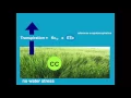
this part of module one focus on the calculation scheme of aquac crop in aquac crop crop yield is simulated in four steps step number one crop development in Step number two crop transpiration is simulated step number three biomass production and finally yield formation in step number four so let's start with the crop development when simulating crop development aquacrop describes the development expansion of the canopy cover which is above ground as well as a development of the root zones which is below the ground a lot of models use Leaf area index aquacrop does not use Leaf
area index but use green canopy cover CC cc is the ratio between the so surface covered by the green canopy cover over the unit ground surface when the sun is directly above the crop you will see on the so a shadow here indicated in purple that is the so surface covered by the green canopy and CC is the ratio of the so surface is covered by the green canopy over the unit ground surface so it ranges from zero when we have a bare so to one when you have full canopy cover or normally it is
expressed in percentage from 0 percentage to 100% here we see the canopy development in function of time in of winter wheat in Belgium the wheat is sound before winter at the end of October and at germination you hardly can see the crop the canopy cover is only 3% after the winter early spring the canopy starts to develop and on the 16th of March it was noted that we have 90% canopy cover one month later already the canopy cover reached already 75% and one month later we are already at 90% canopy development for non-limiting conditions is
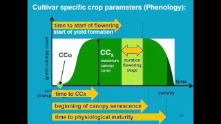
described in aquac crop with only a few crop parameters we have to know the moment when the maximum canopy cover is reached and then by means of a logistic type equation aquac crops describe the development of the canopy between germination and the moment maximum canopy cover is reached at the end of the season uh when senance kicks in the canopy cover will decline so with a few parameters uh which are crop characteristics which is an input uh aquac crop knows how the crop develop under non-limiting conditions throughout the season the conditions are not necessarily non-limiting
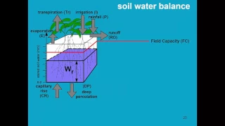
for example water stress in the root Zone might limit canopy development to describe water stress aquac crop simulates the so water balance in a schematic way the root zone is depicted as a Reservoir in which the water content will vary depending on the input and output of water if there's a lot of rainfall or irrigation the water content in the root Zone will increase and will come above Field capacity this will result in deep percolation in the absence of rainfall and irrigation the water content in the root Zone will drop and the crop becomes under
stress when witing point is reached the crop will die now to describe the effect of water stretches on canopy development Aqua crop consider various thresholds the first threshold is a threshold for Le expansion which is indicated here by the green line as soon as the water content drops below the green line the crop experience water STS resulting in a slower Leaf expansion than described by the crop parameters there is a second threshold canopy senon given by the yellow line which is close to wieling point if the water content drops below the yellow line the canopy
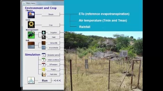
start to die off let us have now a look how canopy cover is simulated in aquac crop when you start aquac crop you get the main menu main menu consists of two panels in the top panel the environment and the crop is described what type of climate we are what is the crop what how is the management on what soil to crop is simulated in the bottom panel we have several options to change the simulations and there is the Run button which I'm going to click now to start the aquac crop now I'm here in
the simulation run and I will start the simulation by clicking on the start button I will advance by 10 days 10 days I continue another 10 days I continue and I continue so my simulation has advanced 40 days in the Run menu I can see three panels one Dr is for crop transpiration one cc is for the canopy development and 1 Dr is the root Zone depletion panel in the rootone depletion panel I can see that the water content has declined we can also see that the root zone is expanding the reservoir becomes bigger but
the amount of water which is given by the blue part is declining now we have several threshold as you remember there is that green line and that is the threshold for canopy expansion it means if the water content drops below the green line then the canopy expansions will slow down and that is what we can see here in the second panel the CC panel where the green canopy cover is simulated in Gray is indicated how the canopy cover should have been developed if there was no water stress however due to water stress the canopy expansion
slows down as soon as the soul water content drops below the green line and it slows down so much that even the canopy expansion is stopped around day 30 now if I irrigate for example I will add 150 mm of water and now I'm going to advance with one day if I click now on continue that water is added in the root Zone I am above Field capacity and immediately the canopy cover starts to increase if I continue my simulation the excess water drains out of the root Zone but canopy is still at full speed
now when I drop below the Green Line canopy cover starts to slow down again and if I'm too far below the green line it even stops now if I continue the water content in the root Zone will drop below the yellow line and Sison starts kicking in and we see that the canopy cover uh dies off and at day 110 I have no longer any canopy cover in Gray it is indicated how the canopy cover should have developed while in green the real canopy cover is uh simulated how it develops in this particular environment when
starting a simulation you select a crop and you know how the canopy development will be for non-limiting conditions as well as how the root development should expand when there are no water stresses at runtime aquac crop will detect water stresses by simulating for each day the so water balance if the water content in the root Zone drops below the green line Leaf expansion will slow down if it drops below the yellow line canopy senance will kick in by considering the stresses at any day of the Season aquac crop will simulate the canop the actual canopy
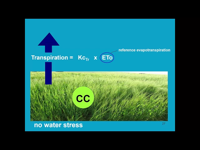
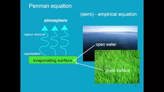
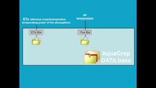
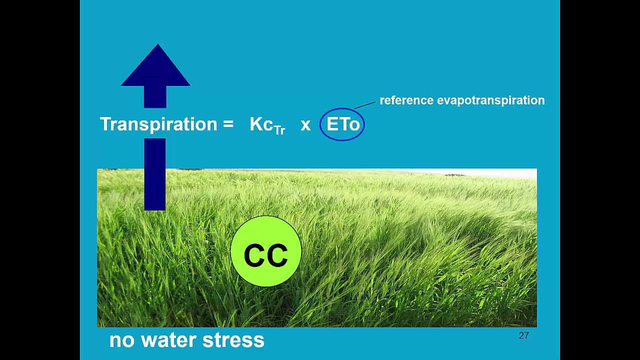
Dev development the same is true for the root development where other stress levels determines the root Zone expansion so this conclude the description of the simulation of canopy cover in Step number one after the simulation of crop development in Step number one we move now to the simulation of crop transpiration in Step number two crop trans insiration consist of the vaporization of liquid water and the vapor removal to the atmosphere it is proportional to CC to simulate transpiration aquacrop uses the KC ET node method eote is reference evapor transpiration it explains it expresses the evaporating
power of the atmosphere which is dictated by the weather conditions and it multiplied with a KC KC is a crop coefficient which characterize the transpiring crop the crop Co efficient is proportional to CC to the green canopy cover when we have a lot of canopy KC will be large and transpiration will be large when cc is small KC is small and transpiration is limited so the KC is proportional to the green canopy cover and the proportional Factor depends on the crop type and expresses how the transpired crop differs from my reference grass crop this is
the simulation of transpiration when there is no water stress so knowing the canopy cover in step one we can now simulate the transpiration by multiplying ET node with a KC factor which is proportional to uh CC see however water stress might close stomata this is simulated once again by considering the soul water balance we have already two thresholds one with the green line expressing use it for simulating leaf expansion and the one with the yellow line use it to simulate canopy sisin we will add now a third threshold which is the one for statal closure
as soon as the soul water content drops below the red line stomatal start to close and transpiration is reduced this is simulated with the help of a water stress factor a KS Factor so when the water content in the root Zone drops below the red line KS becomes smaller than one and transpiration is limited when witing point is reached KS become zero and transpiration is zero so let's return to our aquac crop simulations in which we simulated water stress and after 40 days the canopy development was completely stopped let's now focus on the top panel
the panel for crop transpiration in Gray it indicates how much water could have been been transpired given the actual canopy development however we see starting at day 30 the water content dropped below the red line the red line was the threshold for stomatal closure and the transpiration uh starts to be reduced after applying 150 mm of water and advancing my simulation with a Time step of one day the canopy starts to expand again and transpiration is optimal as soon as the water content drops below the green line the water stress limits canopy expansion which is
explained which is given here canopy expansion reduc it by 1% although the stomatal closure is not affective because the water content is still above the red line it's only when the water content drops below the red line then stomata start to close and I have a reduction of 1% in transpiration if I continue the water content will drop below the yellow line early senance kicks inene and stomata is now already closed by 80% if I continue my simulation my conopy will die off at day 110 far before the end of the growing season so in
the graph of transpiration in Gray it shows me how much water could have been transpired given the green canopy cover however the real transpiration is indicated in blue and is less due to stomatal closure after the simulation of crop development and crop transpiration let's now focus in Step number three on the biomass production crop takes up Water by the roots and that water is transported to the leaves where it escapes as water vapor through the stomata now this same pathway is used to take up CO2 and by photosynthesis the CO2 will be converted in carbohydrates
which are the building blocks of the biomass so we see there is a direct link between crop transpiration and biomass production so when we have a welldeveloped crop nonwater stress a lot of water will escape through the stata and at the same time a lot of CO2 can be taken up when the crop canopy is small and the crop is water stressed transpiration will be small as well and biomass production will be limited as well now the direct relationship between transpiration and biomass is given by the biomass water productivity which gives the slope of the
line in the transpiration biomass curve so when in the first month a certain amount of water is transpired given the slope of the line the biomass production is known if in the second month the crop is poly developed water stress limits the crop transpiration and less biomass is produced in month number three there was a lot of rainfall the crop could develop strongly it transpired a lot and also a lot of biomass was produced in these slides we see for several crops the linearity between the cumulative amount of water which has been transpired and the
biomass production in yellow for sorum in green sunflower blue for Shiki and red for wheat each time we see a linear relationship although the slopes of the lines are different the slopes of the line expresses the water productivity now the slope of the line does not only differ between the crops but also between different climates so in different climates in more colder temperate climates for example the slopes of the line will be different than in more tropical climates therefore aquacrop does not use water productivity as such but he will normalize the water productivity for the
climate that normalization is done by dividing the daily amount of water transpired by the daily amount of e node so the the cumulative transpiration corrected for et node is plotted versus the biomass and once again we see straight lines the yellow line for sorum of course the slope in the normalized graph is different than in the non-normalized graph secondly we will see that crops will group The Green is for the sunflower the red was for the wheat and the blue is for the SHP and we see that the crop they group together in classes we
have a water productivity normalized which is typical for C3 which is lower than the normalized water water productivity for the C4 crops this slide shows you the normalized water productivity for maze in different environments in those environments the climatic conditions are different and also different varieties of maze might have been cultivated nevertheless we found that the normalized water productivity in all those climates in all those environment is very similar so given the amount of water transpired in step two we can calculate the biomass production by knowing what is the water productivity for the crop it
is the normalized water productivity for the crop and so we calculate in Step number three the amount of biomass produced Let Us return to the simulation in aquac crop so far we have discussed the canopy development and crop transpiration as the simulation advances the user can see at the top of the screen the variation in the daily biomass production if transpiration is large the biomass the daily biomass increase is large if transpiration is small the amount of biomass produced on one day will be smaller as well the last step in the calculation scheme of aquac
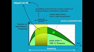
crop is yield formation the simulated above ground biomass integrates all photosynthetic products which were assimilated by the crop during the season by using a harvest index which is a fraction of the biomass that is the harvestable product crop yield is obtained from the biomass with the help of a harvest index aquac crop will derive crop yield from the biomass during the season the Harvest index might vary from its reference value the variation depends on the timing and the extent of water and heat stresses when returning to the simulation run in aquac crop we will find
the final crop yield which was produced at the end of the season at the top of the screen to summarize this presentation we can clearly see in this slide that aquac crop simulates crop yield in four steps step number one canopy cover when canopy cover is known transpiration is simulated by considering the CC biomass is derived from transpiration with the help of the normalized water productivity finally in step four crop yield is derived from biomass by means of the Harvest index