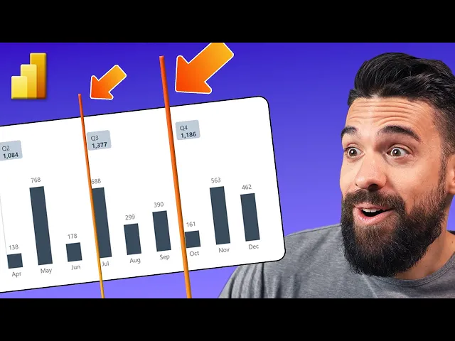
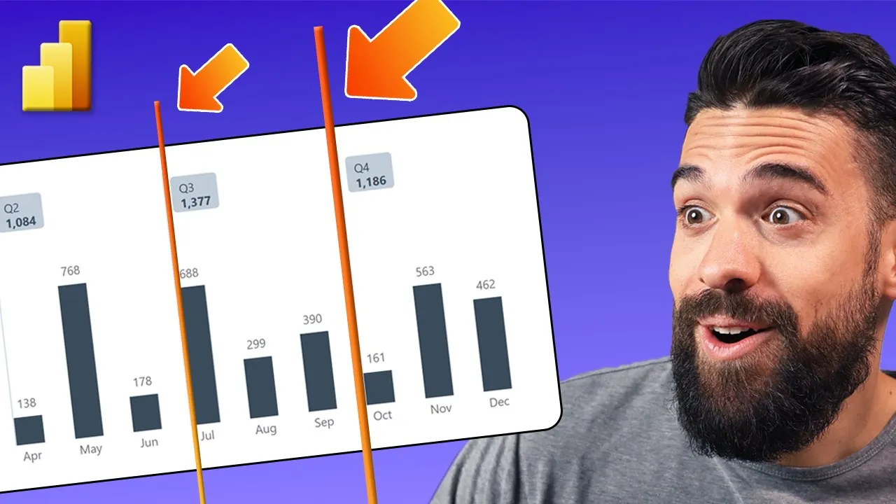
A super helpful PowerBI design trick is to know how to take more control over the vertical lines in your PowerBI visuals to build charts like this one over here where you have a custom separation between different sections of your visualization like quarters where you can then show more information. Now, in this video, I'm going to show you step by step how to set it up. Let's dive in.
As a very first step, let's build this visual over here where we have vertical lines on the left hand side of each column that go all the way to the top where you can put extra information like percent of total or the month overmonth growth rate. All right, now let's go to our starting point. The first thing that we're going to try out is to apply error bars to the series that is visualized which is over here the total number of social media likes.
All right, so I'm going to go to formatting options. Then all the way down there we have arrow bars. if you have under preview options the onob object formatting turned on otherwise you still have to toggle to the analytics tab okay now I'm going to go over here to error bars I'm going to enable it then we have to say what is the upper bound and for that I actually already wrote a measure which is called monthly max now this measure uses a max x function to find the maximum at the month level so it iterates over all of the months which is the granularity that we have in the visual then calculates for each month the number of likes returns the maximum and multiplies that maximum by a random number 1.
65. Now if I use that one for the upper bound of arrow bars let's see what happens. So I'm going to click on add data for the upper bound then look for my monthly max measure.
There it is. And ta we have arrow bars that go all the way to the top. However, I want them to start at zero.
And for that I have another measure, a dummy measure which just returns zero. So that's this one over here. So that it starts on the horizontal x-axis.
Now then we can adjust the formatting. For example, for the bars, I don't want to have a border. So that one I turn off.
And the markers I also turn off. Let's then also make them a little bit lighter. So that's a bit prettier.
And now we already have our vertical lines that go all the way to the top where we can show additional information like the percentages of the total. However, these vertical lines, they cut through the other labels, which is from a design point of view, not so nice. So, what I want to do is take those lines and push them to the left or to the right.
I want to take more control over the vertical lines. Now, how can I do that? Well, to be able to do that, we should not apply these arrow bars to the main series, but to an additional series that we're going to add.
So, I'm going to turn them off again. Now, from the data bane, we take that monthly max measure from before and we're going to add it right above our main measure, the total number of likes. Now, that gives us an extra column series with a constant value.
Now, of course, we don't really want to show these columns. So, we go back over here to formatting columns and then layout where we can make them overlap. Now, then we can play around with the space between the series.
So for example, if I put this to 50%, you see they start to overlap. Now the same for the space between the categories, we can play around with if we want these columns to be a little bit thinner. Now to not show that second series for the monthly max, we go over here to series, select the monthly max, and then set the transparency to 100%.
And now that we have this, we can apply the arrow bars to that second series, the monthly max. So let's enable them. And now set the upper bound to the monthly max.
And then just like before, the lower bound we can set with that dummy zero measure. All right. And then it's just a matter of formatting again.
So here for the bar, I don't want to have a border. So I put that to zero. The bar color I'm going for light blue.
And then here the markers I want to turn off. Now a little bit of fine tuning is needed. So we can go back to columns and then here select again all then layout there we can play around with the space between the series to move these vertical lines to the left hand side of each column.
Now and then for the data labels well those we can change from here data labels then select the series monthly max. And here we simply go to value and set the value not with the monthly max but with a different measure like the percentage of the total or the month over month percentage. And that's it.
Now you can play around with the formatting again. So let's go for a different color. Maybe that dark blue color.
Let's make it bold. All right. Let's make it a little bit smaller.
Let's also change the color of the columns. So go to likes and make it dark blue. Just like this.
Now for the data labels there at the top we of course want to show a different value not that constant value. So if we go back to data labels and then select the monthly max. Well here we want to set the value of the data label not with the monthly max but a different measure like the percentage of total or the month of a month growth rate.
So and now we have their nice percentages for which of course we can also change the formatting a bit maybe to that same color blue. Let's make it bold. All right.
And there you go. Now, if I would like these percentages to be a little bit more to the right. Well, then we can kind of repeat the same trick with an extra measure.
So, I can go back over here to my data field. Take monthly max 2. All right.
Then place this one in between the monthly max and the likes. There you go. And you see we have extra columns.
Not those columns we simply make transparent again. So go back to columns monthly max 2 set the transparency to 100%. All right.
And then we go over here to data labels and do not apply it to the monthly max but the monthly max too where we can just do the same trick. So over here let's change this to percent of total and set the color to light blue. Make it bold.
And if we want the vertical lines to touch the columns, well then we go back here to columns, make sure that all is selected layout and then adjust over here the space between the series. So in this case, we have to set it to 50%. And that's it.
As a next step, I want to take even more control and turn what we have into this over here where we have a separation by quarter. So a vertical line for the start of each quarter with the total for that quarter, the total number of social media likes there at the top in the label. All right.
Now it just requires a few more extra steps. So let's go back to our visual. The first thing that we're going to do is to make sure that we have only one vertical line at the start of each quarter for the columns January, April, July, and October.
So for that I prepared already a measure which only returns the monthly max that other measure under a certain condition and that condition I specified here at the top. Now there I just check the month in the field the context and if it's the first one, fourth one, seventh or 10th one only 10 I return the maximum. That's it.
All right. So then we can use that measure for the error bars. So if I go back to formatting error bars here we have the monthly max series and the upper bound I'm going to set with that new measure.
So monthly max start quarter and then I kind of want to do the same thing for the data labels only return the value for the data label if it is the starting month of a quarter. So let's go over here to our measures and here I prepared a measure data labels value which only returns the quarter when a certain condition holds and that condition is exactly the same as in the previous measure and this measure we can then use to set the data label value. So let's go to the formatting options then data labels.
Now we want to change the data labels for monthly max 2. Then we can open up the value options. Here we have the measure that sets the value which in this case is now going to be that new measure data labels value and it just shows Q1, Q2, Q3, Q4.
Oh, nice. And now I can add more information to it. So here we have detail.
All right, let's enable it. Open it up. Click on data.
And also for the detail part of the label, I created a new measure data labels detail. And this measure is set up in a very similar way. It only returns the quarter value which is calculated over here under a certain condition and it format it in this way.
That's it. All right. So I'm going to go back to the formatting options.
I just want to change the formatting to dark blue color. And let's make the detail values bold. And then here the normal values that show the quarter.
Well, those I want to have in that same color. And let's make it not bold. Maybe also a little bit smaller.
Just like this. And let's change also the background. Let's turn it on.
All right. And let's go for a light blue color. Now, I think this already looks good, but I think it would be even better if we take these labels and push them a bit more inwards so that they are on the right hand side of these vertical lights.
And you can do that if you go here to the build panel and just shuffle around the order because the labels they are applied to well monthly max too. So that one I'm going to push over here to the right hand side. And by doing that you see that the x-axis labels are also nicely lined up with the middle one, the main series number of likes.
And now we just have to well push the vertical lines to the left hand side which we can do by going back to formatting options columns all layout. And then here we can play around with the spacing between the series. So this one I've put now to 16%.
Now let's also push this one a little bit more down. Well now it's all the way at zero. And then I go back to space between series.
And you see with 23% I have the vertical lines nicely aligned on the left hand side of the first column of each quarter. All right. Now if we go back to data labels there's one more adjustment that I would do.
Let's switch to all options. Now here we can still change the position from auto to inside end. You see now they jump inwards more to the right hand side of each vertical line.
However the first one disappeared. So I have to turn overflow text on and then I have them all back again. And another thing I would change is here on the layout.
We have now multi-line and I probably would align the text to the left and side so that they more look like flags. So we have here data label flags as I call it. So you see this is a really nice trick to take more control over the vertical lines in your PowerBI visuals which you don't have with the standard grid lines.
So, if I go here to the grid lines option, you see I cannot even add vertical grid lines to this setup. And what do you think? Do you like this trick?
Let me know in the comment section below. And if you want to learn more PowerBI tips and tricks, then check out these two videos over here. And if you want to build full PowerBI reports with me, learn all of my PowerBI tips of how to build really solid reports every single time, then check out my PowerBI design transformation program.