"The n-body problem is the problem of predicting the individual motions of a group of celestial objects interacting with each other gravitationally. " I'll write my implementation in rust although you should be able to implement it in any Turing complete language. Let's begin by defining what a "celestial object" is.
Every celestial object, or let's call them body, will be a position in space with some velocity, acceleration, and mass. After we've created a new function for the bodies, we can move on to the simulation struct, which will house and handle our world. Here's the way I choose the positions and velocities for the bodies.
This is way beyond the scope of today's video, but I will show you it anyway for completeness' sake. This function is designed for large amounts of bodies - amounts of bodies that we will not be able to simulate, in real time, in this video. Although we're getting ahead of ourself.
Let's move on to the next part of the sentence; "interacting with each other gravitationally. " The force that one body feels from another is equal to the product between the gravitational constant, both masses, the inverse square of the distance between them, and finally the unit vector pointing from the first body towards the source. And, we'll begin by substituting in the equation for the unit vector.
The gravitational constant is incredibly small in reality. It would require either colossal masses, microscopic distances or long stretches of time to observe any significant interaction. Instead, we will set our simulations gravitational constant to one, which not only resolves those issues but also allows us to ignore it entirely.
To calculate the resulting force, we must sum these individual forces towards all other bodies. In other words, we allow the index j to range over the entire bodies vector making sure that j does not equal i, because we do not want a body to accelerate towards itself. To calculate the acceleration for each body we need to divide their resulting force by their mass giving us this expression, which we can simplify by distributing the division over the summation.
Now that we have this equation, we'll apply it to each body at the beginning of every update, allowing us to move on to "predicting the individual motions of a group. " There is in fact an exact analytical solution to the two-body problem given a starting state and some time into the future. This means that it is a solved problem.
On the other hand, the three-body, four-body, or in general, the n-body problem does not have such a solution, and therefore we will have to numerically approximate it. What we want, is a way to take the current state of the system, that is the positions, velocities, accelerations, and masses, and in some way calculate how the system would look a small step into the future. And then do so over and over again.
So let's take a step back and look at what we've got so far. We know the position at the current point in time and we know how to calculate the acceleration using that position, but what is acceleration really? Well, it's the derivative of velocity with respect to time, but we're going to replace this perfect analytical dv/dt with a numerical approximation of the derivative.
You might know that if we were to take the limit as delta-t goes to zero this would be exactly equal, but numerically, in a computer, we're going to just pick an arbitrarily small delta-t as our approximation. The closer it is to zero the better the approximation but also, as you'll see later, the more computationally expensive it will become. Delta-t is also going to be constant so we can improve the notation by replacing t with subscript n and t plus dt with subscript n plus 1.
You can think of n as the current state and n plus 1 as the next. Solving for the next velocity, we get a really nice update rule that we can use to move from one states velocities to the next. Doing a similar derivation with the fact that velocity is the derivative of position, we end up with these two equations, and we can put them to use in a function for the bodies called update.
We also need to reset the acceleration after this as to prepare it for the next frame. After we've calculated their accelerations in the simulation update, we can run their individual updates. If we launch the simulation now, we see that bodies are flying everywhere at very high velocities.
And the issue is that the distance between bodies sometimes happens to very close to zero which means that the acceleration becomes very large. There are multiple ways to solve this but my preferred approach just doesn't allow the distance to become too small. This final magnitude is used to normalize the r vector and therefore should not be limited.
And running this now, we see that it works. But, it isn't very fast. To show this better, I made this graph.
On the horizontal axis, is the amount of bodies, n, and on the vertical axis, is the amount of time, in milliseconds, that an update with that amount of bodies takes on average. As you can see, the curve is clearly quadratic and that means that if you double the amount of bodies, you quadruple the time it takes. I won't go into how to remove this quadratic relationship, in this video, but we can still cut the time per update in half with one simple trick.
To begin, we need to identify the problem, and all you really need to know is that the calculation of acceleration is what's taking up the majority of the time. First of all because square roots are just slow, and second of all because it's in the center of a nested loop. There's nothing inherently wrong with nested loops but because we're trying to increase the amount of bodies as far as possible and both loops depend on the amount of bodies they start to take more and more time really fast as n increases.
We're doing n - 1 acceleration calculations in the inner loop which results in n * (n - 1) calculations for the full loop. This means that this algorithm has the time complexity of O(n^2), which is why the graph looked like n^2 before. To begin optimizing, we should probably look at it in a more visual form.
Here, each box represents an element in the bodies vector, and each arrow represents a calculation of acceleration. What we need to notice is that when we calculate the acceleration from one body towards another and then that other body towards the first body we're using the same distance but we're using the square root to calculate it twice. What we want is to be able to calculate the distance once and then use it to accelerate i to j and j to i at the same time, so let's just try that and see what the consequences are.
The problem now, is that we're accelerating zero to one and then in the next iteration of i, we're again accelerating zero to one, but because we've also already accelerated one towards zero in the previous iteration of i, we can just skip this iteration of j. In the next iteration of i we see the same thing but with both zero and one towards two. And again we can just skip them because we have already calculated them in the previous iterations of i.
This means that we just have to start the iteration of j at i + 1 instead of zero. We have halved the amount of square roots and and that lines up perfectly with what we see in the graph. You might've noticed that there's something I've glossed over, and that's how this vector of bodies in the simulation became a window on the screen with circles flying around and for that, I'll have to send you to my last video, where I went over exactly that and a bit more.
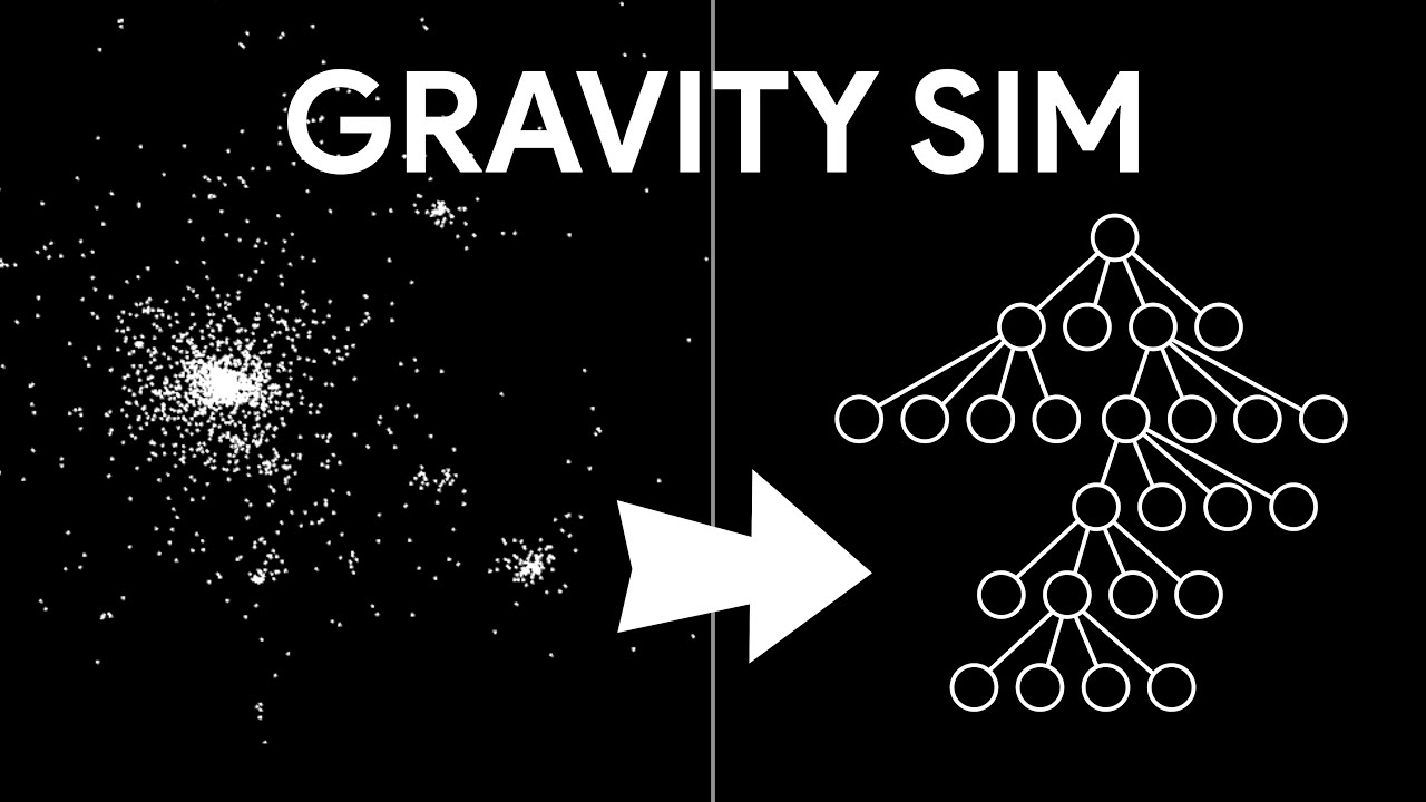
There's still a lot I'd like to add to the simulation, for example, I'd like to implement the Barnes-Hut algorithm to reduce the time complexity from O(n^2) to O(n * log n), but I'll leave that for the next video and until then, thank you for watching, and goodbye.