00020

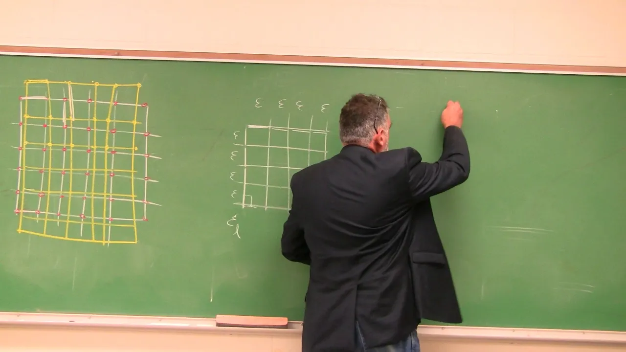
so let's assume that in the first picture this is what the grid looks like and I'm going to use yellow to show what the the grid is going to look like in the second economic saturating and again that I'm messing up the drawing here but you get the idea the idea is that the pattern is going to be distorted some up to pictures the same exact grid one before deformation one after the formation you can go ahead and using for the one picture at a time in ms paint or photoshop measure determine the coordinates that

pixel coordinates of the lumps 1 to 1 to 25 so you measure with the mouse and using the zoom feature the pixel coordinates of the 25 intersection points that define the grid in the first picture put that in an Excel spreadsheet then you go you take the other picture and for the same points you measure the pixel coordinates of the same 25 intersection point 25 nodes I thought you and someone so now you can measure for each of these sites the original length and the deform layer initial length finally for each of the vertical lines

you can measure the initial length the final length so what you can do is the follower for each of these 25 those you're going to be able to measure for this line epsilon for this line epsilon for this epsilon for this epsilon for this epsilon for this and epsilon for this so you're going to be able to measure the change in length for the each of the segments of the horizontal line you will also be able to measure the strain on each of the vertical segments there are one two three four five six well let's

see how many we have here should be five notes there should be five notes and four seconds since there are five notes there are four segments so I'd like to get drawn here a little bit larger one two three four five notes and one two three four five notes so that's the grade that because you're going to have four segments for example four segments with our bird so using the five notes that define each horizontal line you are going to be able to measure the strain along this line for each segment and the average for

the entire line this represents epsilon transfers you can measure along each segment in the vertical direction the change in length and the strain this way and the average which represents longitudinal strain you can measure longitudinal strain along this line along this line along this line along this line and along this one likewise you can measure transverse strain along this line this line this line is line and this one now I hope that by now you get the idea that this is not something that you can do by hand and I don't expect you I don't

want you to do by hand this is the case where you need to use programming in Excel to actually put in the coordinates and once you do that once you do the programming it's really easy and straightforward to get all the information in that one so you simply put in the coordinates of the 25 points before it information from the first picture the 25 coordinates for the points after the formation and then you program in the Excel spreadsheet the requirement evasions to get strain on each of these seconds and then the average for the entire

line the second strain in each of these segments and the average for the entire line and so on so here's an example of how with two pictures and the processing of the images two pictures you are able to measure strain everywhere on one two three four you know sixteen lines and another 16 lines 32 lines you're pretty much able to measure a longitudinal strain transfer strain throughout the picture furthermore you can use the fact that the angles here are 90 degrees or very close to 90 degrees through chain use the change in angle any change

in angle between these two lines to determine the shear strength you remember that the shear strain is defined if this is a 90 degree angle this we call alpha this we called beta gamma physical alpha plus beta the change in angle so that they use it this way the white lines represent the designs before deformation the yellow lines or the orange line sorry represents the same lines after the information so the 90 degree angle because of deformation becomes less than 90 degrees for example or it would become larger 90 to 90 degrees gamma is shear

strength so by measuring the change of angle between these two lines you can measure the shear strain in this location at this point now I want to remind you that if you have a coordinate system that looks like so this is the first quadrant this is the second quadrant this is the third quadrant and this is the fourth what if you have positive shear strain then these angles become as such so this line becomes asaji and this line becomes as such which means that in quadrant one and in Quadrant three the 90 degree angle becomes

less than 90 degrees for positive shear strength whereas in quadrants two and four positive shear strain so gamma larger than zero positive shear strength means that the angle becomes less than 90 degrees in quadrant one and three and larger than 90 degrees C larger than 90 degrees in quadrants two and four so this picture shows positive shear strength that's the shear that were tangled information the scissoring corresponding to both a shear strength in quadrants one and two the 90 degree angle becomes lower less than 90 degrees in quadrants two and four the 90 degree angle

becomes larger than 90 degrees now how can we use that and the grid that we start with to actually measure shear strain and every single one of these points well it's very simple here's what we're gonna do we're going to use something that you remember from vectors you remember that if you have a vector a sorry let's say a vector a well let me make sure that I don't represent any particular situation I present the general case so let me take a vector a and the vector B you remember that a dot product b is

equal to the magnitude of a time's the magnitude of B times cosine of theta where theta is the angle in the tool which means that cosine of theta can be computed as the dot product a dot B divided by the magnitude of a time's the magnitude of B now you remember that if you have a coordinate system you can say that a is equal to ax times I plus a Y times J and B is equal to VX times I plus B Y and then any dot product P can be obtained as ax BX plus

a yd1 which allows you to compute this and the magnitude of a this is nothing else but square root of AX squared plus 8y squared and the same thing here square root of DX squared plus dy squared so here's how you can compute cosine two theta cosine theta the cosine of the angle between two segments all right which means that theta let me write here